"Demystifying Naïve Bayes: Simple yet Powerful for Text Classification"

Naïve Bayes

Naïve Bayes is, first of all, a classification algorithm that helps us solve classification-related problems. Not only does it assist in classification, but it particularly excels in analyzing textual data. If you are working with text or need to perform tasks like spam filtering or sentiment analysis, applying Naïve Bayes as a baseline model is highly recommended before exploring other algorithms, such as deep learning.

For example, let's say you apply Naive Bayes to a text classification task, and it gives you an accuracy of 96%. On the other hand, if you use a heavy neural network in deep learning, you achieve an accuracy of 96.5%. It becomes evident that going for a complex and time-consuming deep neural network for just a 0.5% improvement in accuracy may not be worth it. Naive Bayes is powerful enough to provide satisfactory results in many cases.

In summary, Naïve Bayes is an effective and widely used classification algorithm, especially for tasks involving textual data. Its simplicity, speed, and reasonable accuracy make it a preferred choice as a baseline model before exploring more complex techniques like deep learning.

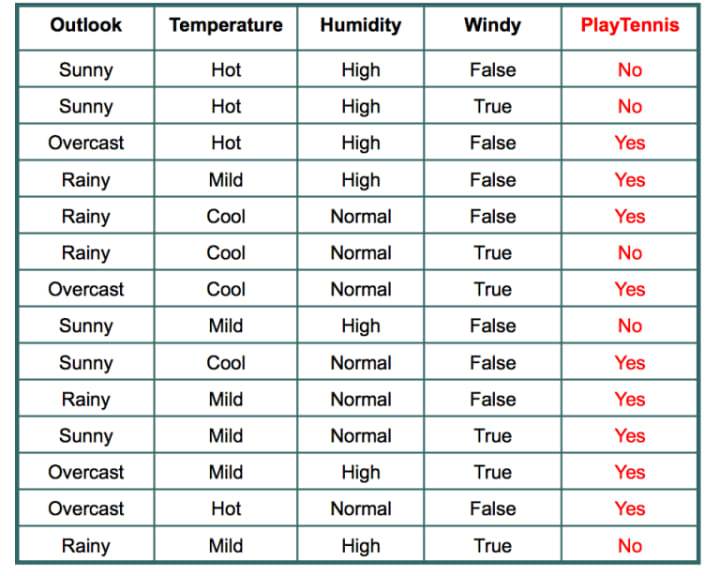
So, over here, what we are going to do is use this simple dataset to understand Naive Bayes. Our goal is to predict whether a student will go to play tennis given these weather conditions.

Let's say we have a query point:

w = {sunny, cool, normal, true}

We need to predict whether the student will go to play tennis (yes or no). We will use Bayes' theorem for this purpose.

The formula is: P(A|B) = (P(B|A) * P(A)) / P(B)

So, our problem formulation is P(yes|w) and P(no|w). Here is the equation:

P(yes|w) = (P(w|yes) * P(yes)) / P(w)

P(no|w) =(P(w|no) * P(no)) / P(w)

By simplifying and removing the denominator from both equations, we can see that they are the same.

The final equation for both probabilities is:

P(yes|w) = (P(w|yes) * P(yes))

P(no|w) =(P(w|no) * P(no)) 

We can easily calculate the probability of "yes" using the given data table, which is 9/14. Similarly, the probability of "no" is 5/14.

However, the difficulty lies in calculating P(w|yes) and P(w|no). Now, we are going to understand how to calculate them given this query point:

w = {sunny, cool, normal, true}

We need to calculate 

(P(w|yes)=P(sunny ∩ cool ∩ normal ∩ true|yes).

(P(w|no)=P(sunny ∩ cool ∩ normal ∩ true|no).

What does it exactly mean?

We need to find the above combination from our data table, i.e., how many times the combination. 

P(sunny ∩ cool ∩ normal ∩ true|yes) 

P(sunny ∩ cool ∩ normal ∩ true|no) 

occurs in our dataset. When we try to find this combination, we may probabilistically encounter a count of 0. This implies that our P(yes|w) will be 0, and the same goes for P(no|w).

This is the problem with Bayes' theorem. When we have lots of input columns, it can sometimes be difficult to find the exact combination of the given input from our dataset. If we cannot find the combination, the probability will be zero.

To solve this problem, Naive Bayes makes a naive assumption. It breaks down the expressions:

P(w|yes) = P(sunny ∩ cool ∩ normal ∩ true|yes) P(w|no) = P(sunny ∩ cool ∩ normal ∩ true|no)

into:

P(w|yes) = P(sunny|yes) * P(cool|yes) * P(normal|yes) * P(true|yes)

Now, you will easily find the above combination in your dataset:

= (frequency of sunny and yes) / (frequency of yes) * (frequency of cool and yes) / (frequency of yes) * (frequency of normal and yes) / (frequency of yes) * (frequency of true and yes) / (frequency of yes)

Similarly:

P(w|no) = (frequency of sunny and no) / (frequency of no) * (frequency of cool and no) / (frequency of no) * (frequency of normal and no) / (frequency of no) * (frequency of true and no) / (frequency of no)

You can try calculating it yourself using the given data table.

So our final equations are:

P(yes|w) = P(sunny|yes) * P(cool|yes) * P(normal|yes) * P(true|yes) * P(yes) = (2/9) * (3/9) * (6/9) * (3/9) * (9/14)

P(no|w) = P(sunny|no) * P(cool|no) * P(normal|no) * P(true|no) * P(no) (Try calculating it yourself using the given data table.)

This is simple intuition behind the naïve Bayes

Let's see what happens during the training phase and testing phase in Naïve Bayes.

During the training phase of Naive Bayes, the algorithm calculates and stores all the probabilities in a dictionary. These probabilities will be used for calculations during the testing phase.

Based on the given example, for the feature "Outlook," we have 3 unique categories (sunny, overcast, rainy) and for the target variable "PlayTennis," we have 2 categories (yes and no). So, the total number of probabilities to be calculated will be 3 x 2 = 6.

For example: P(sunny|yes), P(hot|yes), P(overcast|yes) P(sunny|no), P(hot|no), P(overcast|no) and so on…

The algorithm calculates these probabilities for all the features in the dataset.

So, during the training phase, Naive Bayes computes the probabilities and stores them, and during the testing phase, it utilizes these probabilities to make predictions on new instances.

practical implementation

How Naïve Bayes handles numerical data?

Let's say we have a dataset containing age and marital status information, where we want to predict whether a person is married or not. For example, we have 5 data points in the dataset.

Now, let's consider a scenario where we want to calculate the probability of a person being married at the age of 55. We predict "yes" for married and "no" for not married. So, we want to calculate 

P(yes|55) = (P(55|yes) * P(yes)) / P(w)

P(no|55) =(P(55|no) * P(no)) / P(w)

However, what if we don't have any data points with an age of 55 in our dataset? In that case, both probabilities will be zero because we won't be able to calculate the probability of P(55/yes) or P(55/no).

To handle numerical data in Naïve Bayes, we use a different approach. We assume that the particular age column follows a normal distribution (Gaussian distribution) and calculate the mean (μ) and standard deviation (σ) of the age column.

Now, we can assume that the age values follow a Gaussian distribution. We use the formula.

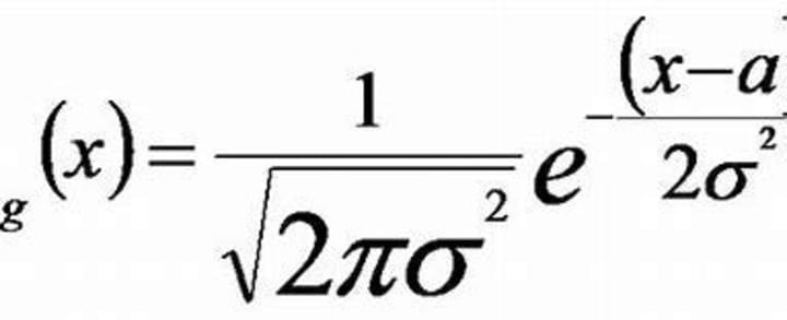
 f(x) = 1 / (σ * √(2π)) * e^(-((x - μ)²) / (2 * σ²)).

 This formula gives us the probability density.

To calculate the probability, we take the query point (in this case, 55) and plot it on our Gaussian distribution. We calculate the probability density at that point, let's say we get 0.62. This means the probability density to get the age of 55 is 0.62 (not exactly the probability, but the probability density).

Gaussian distribution for yes

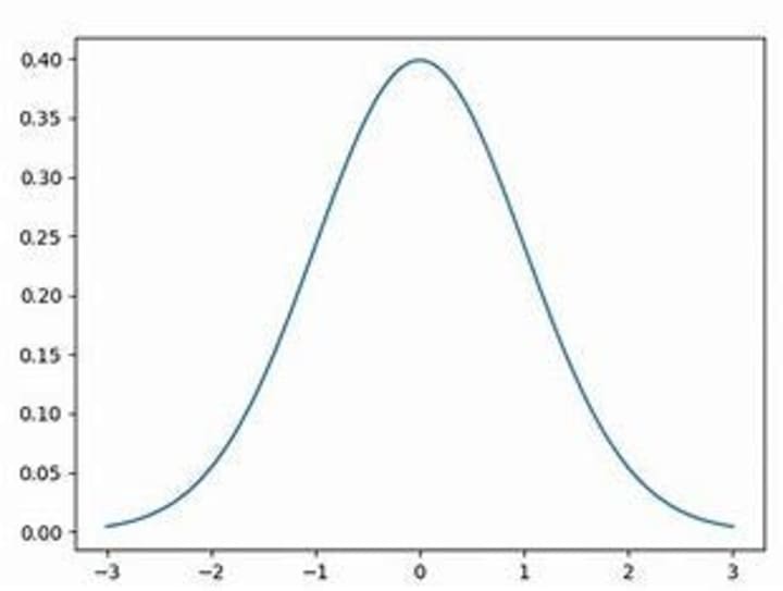
Gaussian distribution for No

It's important to note that for both classes (married and not married), we have two different Gaussian distributions, one for "yes" and another for "no". We calculate the probability density using the respective distribution.

After performing the calculation, we replace P(55/yes) with 0.62. Even though we don't have the exact data point in our dataset, we can calculate the probability using the distribution.

It's worth mentioning that this approach assumes the particular column or feature follows a Gaussian distribution. If the data follows a different distribution, such as a chi-square distribution, we would apply the corresponding formulation for that distribution. If the data doesn't follow any well-known distribution, we would need to explore alternative techniques to handle such cases.

What is data is not Gaussian?

1. Data Transformation: Depending on the nature of your data, you could apply a transformation to make it more normally distributed. Common transformations include the logarithm, square root, and reciprocal transformations. 
2. Alternative Distributions: If you know or suspect that your data follow a specific nonmoral distribution (e.g., exponential, Poisson, etc.), you can modify the Naïve Bayes algorithm to assume that specific distribution when calculating the likelihoods. 
3. Discretization: You can turn your continuous data into categorical data by binning the values. There are various ways to decide on the bins, including equal width bins, equal frequency bins, or using a more sophisticated method like k-means clustering. Once your data is binned, you can use the standard Multinomial or Bernoulli Naïve Bayes methods. 
4. Kernel Density Estimation: A non-parametric way to estimate the probability density function of a random variable. Kernel density estimation can be used when the distribution is unknown. 
5. Use other models: If none of the above options work well, it may be best to consider a different classification algorithm that doesn't make strong assumptions about the distributions of the features, such as Decision Trees, Random Forests, or Support Vector Machines

Naïve Bayes on Text Data

Naive Bayes is commonly applied to text data for tasks such as text classification, sentiment analysis, spam detection, and document categorization. It is particularly suitable for text data due to its simplicity and ability to handle high-dimensional feature spaces efficiently.

Let's consider a real-world example of applying Naive Bayes to text data for sentiment analysis. Suppose we have a dataset of customer reviews for a product, where each review is labeled as either positive or negative sentiment.

The first step is to preprocess the text data by removing stop words, punctuation, and performing stemming or lemmatization to reduce the dimensionality of the features.

Next, we split the dataset into a training set and a testing set. The training set will be used to train the Naive Bayes classifier, and the testing set will be used to evaluate its performance.

During the training phase, the Naive Bayes algorithm calculates the probabilities of each word occurring in positive and negative reviews. It estimates the conditional probabilities of each word given the sentiment (positive or negative).

For example, let's say we have the following reviews:

Review 1: "The product is excellent." 

Review 2: "The product is terrible." 

Review 3: "I love this product."

From these reviews, the algorithm builds a vocabulary consisting of unique words, and for each sentiment (positive and negative), it calculates the probability of each word occurring in that sentiment.

During the testing phase, the trained Naive Bayes model is used to predict the sentiment of new, unseen reviews. The algorithm calculates the probability of each sentiment given the words in the review and selects the sentiment with the highest probability as the predicted sentiment for that review.

For example, if we have a new review "I don't like this product," the Naive Bayes algorithm will calculate the probabilities of this review belonging to the positive and negative sentiment classes. It considers the conditional probabilities of each word given the sentiment and applies Bayes' theorem to estimate the posterior probabilities.

Finally, the algorithm predicts the sentiment (positive or negative) based on the highest posterior probability.

Overall, Naïve Bayes for text data involves estimating the probabilities of words given the sentiment during the training phase and using those probabilities to predict the sentiment of new, unseen text during the testing phase.

Also check out our 2nd and 3rd post on it

link is given in the comment section.