"Unlocking the Power of Chi Square: A Guide to Statistical Analysis"

Chi Square Distribution

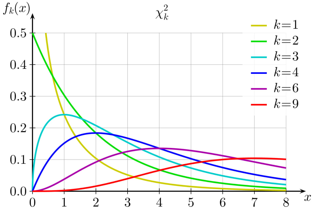
The Chi-Square distribution, also written as χ² distribution, is a continuous probability distribution that is widely used in statistical hypothesis testing, particularly in the context of goodness-of-fit tests and tests for independence in contingency tables. It arises when the sum of the squares of independent standard normal random variables follows this distribution.

The Chi-Square distribution has a single parameter, the degrees of freedom (df), which influences the shape and spread of the distribution. The degrees of freedom are typically associated with the number of independent variables or constraints in a statistical problem.

Some key properties of the Chi-Square distribution are:

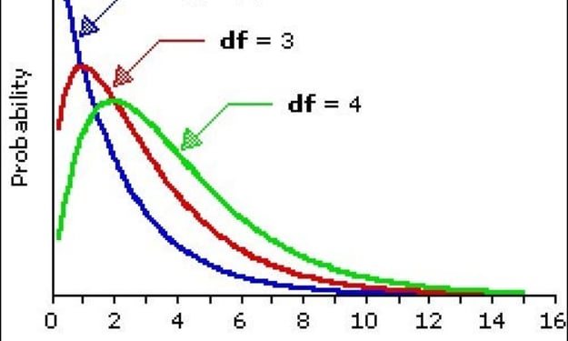
a. It is a continuous distribution, defined for non-negative values. It is positively skewed, with the degree of skewness decreasing as the degrees of freedom increase.

b. The mean of the Chi-Square distribution is equal to its degrees of freedom, and its variance is equal to twice the degrees of freedom.

c. As the degrees of freedom increase, the Chi-Square distribution approaches the normal distribution in shape.

d. The Chi-Square distribution is used in various statistical tests, such as the Chi-square goodness-of-fit test, which evaluates whether an observed frequency distribution fits an expected theoretical distribution, and the Chi-Square test for independence, which checks the association between categorical variables in a contingency table.

---

Chi-square test is a statistical test used to determine if there is a significant association between two categorical variables. It is a non-parametric test, which means it does not make any assumptions about the distribution of the data

It is based on the Chi-Square (χ²) distribution, and it is commonly applied in two main scenarios:

1. Chi-Square Goodness-of-Fit Test: This test is used to determine if the observed distribution of a single categorical variable matches an expected theoretical distribution. It is often applied to check if the data follows a specific probability distribution, such as the uniform or binomial distribution.

2. Chi-Square Test for Independence (Chi-Square Test for Association): This test is used to determine whether there is a significant association between two categorical variables in a sample.

Here's a simple explanation of how chi-square test works along with examples

Suppose you are interested in determining whether there is a significant relationship between smoking and lung cancer. You collect data on 100 individuals and classify them into two groups: smokers and non-smokers. You then count the number of individuals in each group who have developed lung cancer.

To perform a chi-square test on this data, you start by stating a null hypothesis that there is no association between smoking and lung cancer. Then, you calculate the expected frequencies for each cell if there was no association between smoking and lung cancer. This is done by multiplying the row total by the column total and dividing by the grand total:

Next, you calculate the chi-square statistic using the formula:

χ² = Σ (Observed frequency - Expected frequency)² / Expected frequency

The degrees of freedom (df) for a chi-square test with two rows and two columns is 1. The significance level is typically set at 0.05.

If the calculated value of chi-square is greater than the critical value at the 0.05 level, then you can reject the null hypothesis and conclude that there is a significant association between smoking and lung cancer.

---

Goodness Of Fit Test

I'd be happy to explain the goodness of fit test in detail with examples and calculations.

The goodness of fit test is a statistical method used to determine whether a set of data follows a particular probability distribution or theoretical model. The test involves comparing the observed data with the expected data that would be generated by the theoretical model, and assessing whether the differences between the two are significant.

Here are the steps involved in conducting a goodness of fit test:

Step 1: Define the null hypothesis and alternative hypothesis. The null hypothesis states that the observed data follows the specified probability distribution or theoretical model. The alternative hypothesis states that the observed data does not follow the specified probability distribution or theoretical model.

Step 2: Choose the appropriate test statistic. The choice of test statistic will depend on the specific hypothesis being tested and the type of data being analyzed. The most commonly used test statistic for goodness of fit tests is the chi-squared test statistic.

Step 3: Calculate the test statistic. This involves comparing the observed data with the expected data generated by the theoretical model. The formula for the chi-squared test statistic is:

χ² = Σ [(Oi - Ei)² / Ei]

Where: χ² = Chi-squared test statistic Oi = Observed frequency for category i Ei = Expected frequency for category i

Step 4: Determine the degrees of freedom. The degrees of freedom for the chi-squared test statistic are calculated as the number of categories minus 1.

Step 5: Determine the p-value. The p-value is the probability of obtaining a test statistic as extreme or more extreme than the one calculated, assuming the null hypothesis is true. This can be calculated using a chi-squared distribution table or a statistical software program.

Step 6: Compare the p-value to the significance level. If the p-value is less than the significance level (usually set at 0.05), then the null hypothesis is rejected. This indicates that the observed data does not follow the specified probability distribution or theoretical model. If the p-value is greater than the significance level, then the null hypothesis cannot be rejected.

Assumptions:

1. The data is independent and identically distributed (i.i.d).
2. The data is drawn from a random sample.
3. The expected frequencies for each category are greater than or equal to 5.

Now let's look at an example of how to conduct a goodness of fit test:

Example 1: Suppose we have a sample of 100 people, and we want to test whether their blood types follow the expected frequencies of the ABO blood group system (A, B, AB, O), which are 0.41, 0.10, 0.04, and 0.45 respectively. The observed frequencies for each blood type are:

Step 1: Define the null and alternative hypotheses.

Null hypothesis: The observed frequencies of the blood types follow the expected frequencies of the ABO blood group system.

Alternative hypothesis: The observed frequencies of the blood types do not follow the expected frequencies of the ABO blood group system.

Step 2: Choose the appropriate test statistic. In this case, we will use the chi-squared test statistic.

Step 3: Calculate the test statistic. Using the formula for the chi-squared test statistic, we get:

χ² = [(45–41)² / 41] + [(5–10)² / 10] + [(3–4)² / 4] + [(47–45)² / 45]

= 1.79 + 2.50 + 0.25 + 0.18 = 4.72

Step 4: Determine the degrees of freedom. The degrees of freedom for the chi-squared test statistic are (number of categories - 1), which in this case is 4–1 = 3.

Step 5: Determine the p-value. Using a chi-squared distribution table with 3 degrees of freedom and a significance level of 0.05, we find that the p-value is 0.193.

Step 6: Compare the p-value to the significance level. Since the p-value (0.193) is greater than the significance level (0.05), we cannot reject the null hypothesis. This means that the observed frequencies of the blood types do not significantly differ from the expected frequencies of the ABO blood group system.

Example 2: Suppose we have a sample of 50 customers and we want to test whether their purchasing habits follow the expected frequencies of three product categories (A, B, C), which are 0.4, 0.3, and 0.3 respectively. The observed frequencies for each category are:

Step 1: Define the null and alternative hypotheses.

Null hypothesis: The observed frequencies of the product categories follows the expected frequencies.

Alternative hypothesis: The observed frequencies of the product categories do not follow the expected frequencies.

Step 2: Choose the appropriate test statistic. In this case, we will use the chi-squared test statistic.

Step 3: Calculate the test statistic. Using the formula for the chi-squared test statistic, we get:

χ² = [(19–20)² / 20] + [(14–15)² / 15] + [(17–15)² / 15] = 0.05 + 0.11 + 0.47 = 0.63

Step 4: Determine the degrees of freedom. The degrees of freedom for the chi-squared test statistic are (number of categories - 1), which in this case is 3–1 = 2.

Step 5: Determine the p-value. Using a chi-squared distribution table with 2 degrees of freedom and a significance level of 0.05, we find that the p-value is 0.729.

Step 6: Compare the p-value to the significance level. Since the p-value (0.729) is greater than the significance level (0.05), we cannot reject the null hypothesis. This means that the observed frequencies of the product categories do not significantly differ from the expected frequencies.

Assumptions:

1. The data is independent and identically distributed (i.i.d).
2. The data is drawn from a random sample.
3. The expected frequencies for each category are greater than or equal to 5.

Example using Tetanic dataset.

This code first creates an array of observed frequencies by counting the number of passengers in each passenger class. It then calculates the expected frequencies assuming a uniform distribution of passengers across all classes. It then conducts a chi-squared test of goodness of fit and prints the results, including the observed and expected frequencies, the test statistic, and the p-value. Note that we are only using the Pclass column and not the Survived column in this example.

import numpy as np

import pandas as pd

from scipy.stats import chisquare

# Load Titanic dataset

titanic = pd.read_csv('titanic.csv')

# Create observed frequency array

obs_freq = titanic['Pclass'].value_counts().sort_index().values

# Calculate expected frequencies assuming uniform distribution

exp_freq = np.full_like(obs_freq, fill_value=obs_freq.sum() / len(obs_freq))

# Conduct chi-squared test of goodness of fit

chi_sq, p_value = chisquare(obs_freq, exp_freq)

# Print results

print('Observed Frequencies:', obs_freq)

print('Expected Frequencies:', exp_freq)

print('Chi-Squared Test Statistic:', chi_sq)

print('p-value:', p_value)

Observed Frequencies: [216 184 491]

Expected Frequencies: [297. 297. 297.]

Chi-Squared Test Statistic: 94.11014479902915

p-value: 3.643791545115704 e-21

in the context of a chi-squared goodness of fit test, the null hypothesis is that the observed data fits the expected distribution. The alternative hypothesis is that the observed data does not fit the expected distribution.

In the example code provided, the null hypothesis is that the observed distribution of passenger class in the Titanic dataset follows a uniform distribution. The alternative hypothesis is that the observed distribution does not follow a uniform distribution.

The p-value is very small (much less than the commonly used alpha level of 0.05), which indicates that the observed distribution is significantly different from the expected uniform distribution. Therefore, we reject the null hypothesis of uniform distribution and conclude that there is a statistically significant difference between the observed and expected distributions.

--

Test For Independence

A test for independence is used to determine if there is a relationship between two categorical variables. The null hypothesis for this test is that there is no association between the two variables, while the alternative hypothesis is that there is a relationship. The test for independence uses the chi-squared statistic and is commonly used in social science research.

Here are the steps for conducting a test for independence:

hypotheses: The null hypothesis is that the two variables are independent (i.e., there is no association between them), while the alternative hypothesis is that they are dependent (i.e., there is an association between them).

Set the level of significance (alpha): This is the probability level that will be used to determine if the null hypothesis will be rejected or not. A common value for alpha is 0.05.

Create a contingency table: A contingency table shows the number of observations for each combination of the two variables. It is important to make sure that the sample size is large enough so that the expected frequencies for each cell in the table are greater than 5.

Calculate the expected frequencies: The expected frequencies are calculated assuming that the null hypothesis is true. They can be calculated using the formula: (row total * column total) / grand total.

Calculate the test statistic: The test statistic is the chi-squared statistic, which measures the difference between the observed and expected frequencies.

Determine the degrees of freedom: The degrees of freedom are calculated using the formula: (number of rows - 1) * (number of columns - 1).

Determine the p-value: The p-value is the probability of obtaining a chi-squared statistic as extreme as the one calculated from the sample, assuming that the null hypothesis is true. It can be calculated using a chi-squared distribution table or using statistical software.

Make a decision: Compare the p-value to the level of significance. If the p-value is less than alpha, reject the null hypothesis and conclude that there is a relationship between the two variables. If the p-value is greater than alpha, fail to reject the null hypothesis and conclude that there is no relationship between the two variables.

Here are two examples of conducting a test for independence:

Example 1:

Suppose we want to test if there is a relationship between gender and smoking status. We randomly select 500 individuals and record their gender and smoking status. The contingency table is shown below:

The null hypothesis is that gender and smoking status are independent. The alternative hypothesis is that they are dependent. We will use a significance level of 0.05.

To conduct the test, we first calculate the expected frequencies assuming the null hypothesis is true:

Next, we calculate the chi-squared test statistic:

chi_sq = sum((observed - expected)² / expected) = [(200–180)² / 180] + [(100–120)² / 120] + [(100–120)² / 120] + [(200–80)² / 80]

= 22.08

The degrees of freedom for this test are (2–1) * (2–1) = 1.

Using a chi-squared distribution table or statistical software, we find that the p-value is less than 0.05. Therefore, we reject the null hypothesis and conclude that there is a relationship between gender and smoking status.

Example 2:

Suppose we want to test if there is a relationship between political affiliation and support for a certain policy. We randomly select 1000 individuals and record their political affiliation (Democratic, Republican, or Independent) and their support for the policy (Support or Oppose). The contingency table is shown below:

The null hypothesis is that political affiliation and support for the policy are independent. The alternative hypothesis is that they are dependent. We will use a significance level of 0.05.

To conduct the test, we first calculate the expected frequencies assuming the null hypothesis is true:

SupportOpposeTotalDemocratic275225500Republican137.5112.5250Independent137.5112.5250Total5504501000

Next, we calculate the chi-squared test statistic:

chi_sq = sum((observed - expected)² / expected) = [(300–275)² / 275] + [(200–225)² / 225] + [(100–137.5)² / 137.5] + [(150–112.5)² / 112.5] + [(150–137.5)² / 137.5] + [(100–112.5)² / 112.5] = 19.22

The degrees of freedom for this test are (3–1) * (2–1) = 2.

Using a chi-squared distribution table or statistical software, we find that the p-value is less than 0.05. Therefore, we reject the null hypothesis and conclude that there is a relationship between political affiliation and support for the policy.

Assumptions:

1. Independence of observations: Each observation in the sample must be independent of all other observations.
2. Sample size: The sample size must be large enough so that the expected frequencies for each cell in the contingency table are greater than 5.
3. Random sampling: The sample must be a random sample from the population.

Example 2:

Suppose a researcher wants to investigate whether there is a relationship between level of education and income. The researcher randomly samples 500 individuals and records their highest level of education completed (less than high school, high school diploma, some college, or college degree) and their annual income (less than $30,000, $30,000 to $50,000, $50,000 to $80,000, or more than $80,000). The contingency table is shown below:

The null hypothesis is that level of education and income are independent. The alternative hypothesis is that they are dependent. We will use a significance level of 0.05.

To conduct the test, we first calculate the expected frequencies assuming the null hypothesis is true:

Next, we calculate the chi-squared test statistic:

chi_sq = sum((observed - expected)² / expected) = [(70–38.46)² / 38.46] + [(50–61.54)² / 61.54] + [(30–47.69)² / 47.69] + [(10–12.31)² / 12.31] + [(60–60)² / 60] + [(80–96)² / 96] + [(50–74)² / 74] + [(10–18)² / 18] + [(40–49.23)² / 49.23] + [(60–78.46)² / 78.46] + [(70–60.77)² / 60.77] + [(30–11.54)^

² / 11.54] + [(20–42.31)² / 42.31] + [(50–67.69)² / 67.69] + [(70–52.31)² / 52.31] + [(80–12.69)² / 12.69] = 137.95

The degrees of freedom for the test is (r - 1) * (c - 1) = 3 * 3 = 9, where r is the number of rows and c is the number of columns in the contingency table. We use a chi-squared distribution table or a statistical software to find the critical value of the test statistic for a significance level of 0.05 and 9 degrees of freedom, which is 16.919. Since our calculated chi-squared value of 137.95 is greater than the critical value of 16.919, we reject the null hypothesis and conclude that there is evidence of a relationship between level of education and income.

Assumptions:

1. The observations are independent.
2. The sample size is sufficiently large (at least 5 expected frequencies in each cell).
3. The expected frequencies are not too small (no more than 20% of the cells have expected frequencies less than 5).

Applications in Machine Learning

Feature selection:

Chi-Square test can be used as a filter-based feature selection method to rank and select the most relevant categorical features in a dataset. By measuring the association between each categorical feature and the target variable, you can eliminate irrelevant or redundant features, which can help improve the performance and efficiency of machine learning models.

Evaluation of classification models:

For multi-class classification problems, the Chi-Square test can be used to compare the observed and expected class frequencies in the confusion matrix. This can help assess the goodness of fit of the classification model, indicating how well the model's predictions align with the actual class distributions.

Analyzing relationships between categorical features:

In exploratory data analysis, the Chi-square test for independence can be applied to identify relationships between pairs of categorical features. Understanding these relationships can help inform feature engineering and provide insights into the underlying structure of the data.

Discretization of continuous variables:

When converting continuous variables into categorical variables (binning), the Chi-Square test can be used to determine the optimal number of bins or intervals that best represent the relationship between the continuous variable and the target variable.

Variable selection in decision trees:

Some decision tree algorithms, such as the CHAID (Chi squared Automatic Interaction Detection) algorithm, use the Chi-Square test to determine the most significant splitting variables at each node in the tree. This helps construct more effective and interpretable decision trees.