"Unveiling the Assumptions of Linear Regression: Unlocking the Secrets Behind Accurate Predictive Modeling"

Linear regression relies on several assumptions to ensure the validity and reliability of the estimates and inferences.

Google Collaboratory

The key assumptions of linear regression are:

1. Linearity
2. Normality of Residuals
3. Homoscedasticity
4. No Autocorrelation
5. No or little Multicollinearity.

The Assumption

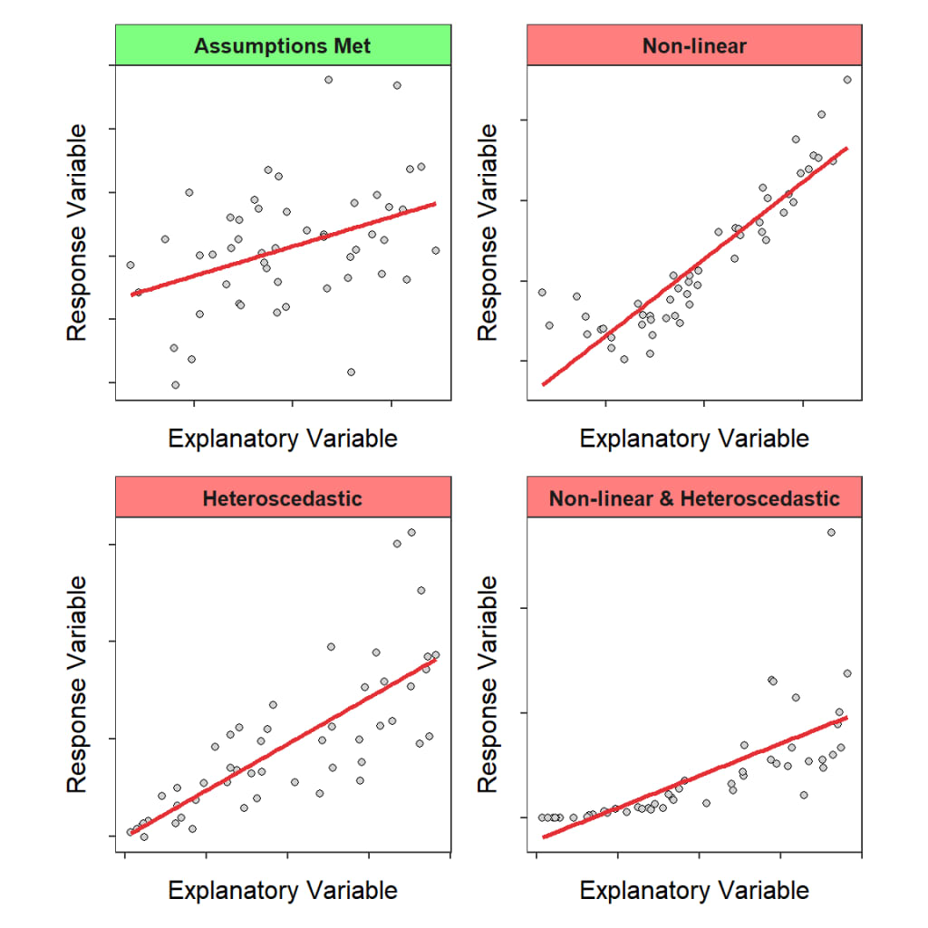
# 1. Linearity

There is a linear relationship between the independent variables and the dependent variable. The model assumes that changes in the independent variables lead to proportional changes in the dependent variable.

What happens when this assumption is violated?

1. Bias in parameter estimates: When the true relationship is not linear, the estimated regression coefficients can be biased, leading to incorrect inferences about the relationship between the independent and dependent variables.
2. Reduced predictive accuracy: A mis specified linear model may not accurately capture the underlying relationship, which can result in poor predictive performance. The model might underfit the data, missing important patterns and trends.
3. Invalid hypothesis tests and confidence intervals: The violation of the linearity assumption can affect the validity of hypothesis tests and confidence intervals, leading to incorrect inferences about the significance of the independent variables and the effect sizes.

How to check this assumption

1. Scatter plots:Create scatter plots of the dependent variable against each independent variable. If the relationship appears to be linear, the linearity assumption is likely satisfied. Nonlinear patterns or other trends may indicate that the assumption is violated.
2. Residual plots: Plot the residuals (the differences between the observed and predicted values) against the predicted values or against each independent variable. If the linearity assumption holds, the residuals should be randomly scattered around zero, with no discernible pattern. Any trends, curvature, or heteroscedasticity in the residual plots suggest that the linearity assumption may be violated.

# Fit a linear regression model

X = df[['x1', 'x2']]

y = df['y']

model = LinearRegression()

model.fit(X, y)

# Calculate predicted values and residuals

y_pred = model.predict(X)

residuals = y - y_pred

# Plot residuals against predicted values

plt.scatter(y_pred, residuals, color='blue')

plt.axhline(y=0, color='red', linestyle='--')

plt.title('Residuals vs. Predicted Values')

plt.xlabel('Predicted Values')

plt.ylabel('Residuals')

plt.show()

3. Polynomial terms: Add polynomial terms to your model and compare the model fit with the original linear model. If the new model with additional terms significantly improves the fit, it may suggest that the linearity assumption is violated.

from sklearn.preprocessing import PolynomialFeatures

from sklearn.metrics import r2_score, mean_squared_error

from sklearn.model_selection import train_test_split

# Split the data into train and test sets

X_train, X_test, y_train, y_test = train_test_split(X, y, test_size=0.2, random_state=42)

# Fit a linear regression model

linear_model = LinearRegression()

linear_model.fit(X_train, y_train)

linear_y_pred = linear_model.predict(X_test)

# Calculate metrics for linear model

linear_r2 = r2_score(y_test, linear_y_pred)

linear_mse = mean_squared_error(y_test, linear_y_pred)

# Fit a polynomial model

poly_features = PolynomialFeatures(degree=2)

X_train_poly = poly_features.fit_transform(X_train)

X_test_poly = poly_features.transform(X_test)

poly_model = LinearRegression()

poly_model.fit(X_train_poly, y_train)

poly_y_pred = poly_model.predict(X_test_poly)

# Calculate metrics for polynomial model

poly_r2 = r2_score(y_test, poly_y_pred)

poly_mse = mean_squared_error(y_test, poly_y_pred)

# Compare model performance

print("Linear model")

print(f"R-squared: {linear_r2:.4f}")

print(f"Mean Squared Error: {linear_mse:.4f}")

print("\nPolynomial model")

print(f"R-squared: {poly_r2:.4f}")

print(f"Mean Squared Error: {poly_mse:.4f}")

Result

# Linear model

R-squared: 0.0954

Mean Squared Error: 30.8182

# Polynomial model

R-squared: 0.9468

Mean Squared Error: 1.8122

You can clearly see after applying polynomial features our accuracy is increased means our linearity assumption is violated.

What to do when the assumption fails?

1. Transformations: Apply transformations to the dependent and/or independent variables to make their relationship more linear. Common transformations include logarithmic, square root, and inverse transformations.

import numpy as np

import pandas as pd

import matplotlib.pyplot as plt

from sklearn.linear_model import LinearRegression

from sklearn.metrics import r2_score

# Generate a non-linear dataset with a quadratic relationship

np.random.seed(42)

x = 10 * np.random.rand(100, 1)

y = x**2 + 5 + np.random.normal(0, 5, (100, 1))

y = np.abs(y) # Ensure y is non-negative

# Apply square root transformation to y

y_sqrt = np.sqrt(y)

# Fit linear regression models for the original and transformed data

linear_model_original = LinearRegression()

linear_model_original.fit(x, y)

linear_model_transformed = LinearRegression()

linear_model_transformed.fit(x, y_sqrt)

# Predictions

y_pred_original = linear_model_original.predict(x)

y_pred_transformed = linear_model_transformed.predict(x)

# Visualize the relationship between x and y before and after transformation

fig, (ax1, ax2) = plt.subplots(1, 2, figsize=(12, 5))

# Before transformation

ax1.scatter(x, y, color='blue')

ax1.plot(x, y_pred_original, color='red', linewidth=2)

ax1.set_title('Original Data')

ax1.set_xlabel('x')

ax1.set_ylabel('y')

# After transformation

ax2.scatter(x, y_sqrt, color='blue')

ax2.plot(x, y_pred_transformed, color='red', linewidth=2)

ax2.set_title('Transformed Data (Square Root Transformation)')

ax2.set_xlabel('x')

ax2.set_ylabel('sqrt(y)')

plt.show()

# Calculate R-squared and Mean Squared Error

r2_original = r2_score(y, y_pred_original)

r2_transformed = r2_score(y_sqrt, y_pred_transformed)

# Compare the performance of the original and transformed models

print("Original linear model")

print(f"R-squared: {r2_original:.4f}")

print("\nTransformed linear model")

print(f"R-squared: {r2_transformed:.4f}")

Original linear model

R-squared: 0.9008

Transformed linear model

R-squared: 0.9291

2. Polynomial regression: Add polynomial terms of the independent variables to the model to capture non-linear relationships.

import numpy as np

import pandas as pd

import matplotlib.pyplot as plt

from sklearn.linear_model import LinearRegression

from sklearn.preprocessing import PolynomialFeatures

from sklearn.metrics import r2_score, mean_squared_error

# Generate a non-linear dataset with a quadratic relationship

np.random.seed(42)

x = 10 * np.random.rand(100, 1)

y = x**2 + 5 + np.random.normal(0, 5, (100, 1))

y = np.abs(y) # Ensure y is non-negative

# Fit linear regression model

linear_model = LinearRegression()

linear_model.fit(x, y)

y_pred_linear = linear_model.predict(x)

# Fit polynomial regression model (degree = 2)

poly_features = PolynomialFeatures(degree=2, include_bias=False)

x_poly = poly_features.fit_transform(x)

poly_model = LinearRegression()

poly_model.fit(x_poly, y)

y_pred_poly = poly_model.predict(x_poly)

# Visualize the fitted lines for linear and polynomial regression

fig, (ax1, ax2) = plt.subplots(1, 2, figsize=(12, 5))

# Linear regression

ax1.scatter(x, y, color='blue')

ax1.plot(x, y_pred_linear, color='red', linewidth=2)

ax1.set_title('Linear Regression')

ax1.set_xlabel('x')

ax1.set_ylabel('y')

# Polynomial regression

ax2.scatter(x, y, color='blue')

ax2.plot(sorted(x[:, 0]), y_pred_poly[np.argsort(x[:, 0])], color='red', linewidth=2)

ax2.set_title('Polynomial Regression (Degree = 2)')

ax2.set_xlabel('x')

ax2.set_ylabel('y')

plt.show()

# Calculate R-squared for both models

r2_linear = r2_score(y, y_pred_linear)

r2_poly = r2_score(y, y_pred_poly)

# Compare the performance of the linear and polynomial regression models

print("Linear regression")

print(f"R-squared: {r2_linear:.4f}")

print("\nPolynomial regression (degree = 2)")

print(f"R-squared: {r2_poly:.4f}")

Linear regression

R-squared: 0.9008

Polynomial regression (degree = 2)

R-squared: 0.9782

1. Piecewise regression: Divide the range of the independent variable into segments and fit separate linear models to each segment.
2. Non-parametric or semi-parametric methods: Consider using non-parametric or semiparametric methods that do not rely on the linearity assumption, such as generalized additive models (GAMs), splines, or kernel regression.

------------------------------------------------------------------------------------

#2. Normality of Residual

The Assumption The error terms (residuals) are assumed to follow a normal distribution with a mean of zero and a constant variance.

What happens when this assumption is violated?

1. Inaccurate hypothesis tests: The t-tests and F-tests used to assess the significance of the regression coefficients and the overall model rely on the normality assumption. If the residuals are not normally distributed, these tests may produce inaccurate results, leading to incorrect inferences about the significance of the independent variables.
2. Invalid confidence intervals: The confidence intervals for the regression coefficients are based on the assumption of normally distributed residuals. If the normality assumption is violated, the confidence intervals may not be accurate, affecting the interpretation of the effect sizes and the precision of the estimates.
3. Model performance: The violation of the normality assumption may indicate that the chosen model is not the best fit for the data, potentially leading to reduced predictive accuracy.

How to check this assumption

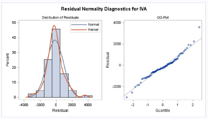
1. Histogram of residuals: Plot a histogram of the residuals to visually assess their distribution. If the histogram resembles a bell-shaped curve, it suggests that the residuals are normally distributed.
2. Q-Q plot: A Q-Q (quantile-quantile) plot compares the quantiles of the residuals to the quantiles of a standard normal distribution. If the points in the Q-Q plot fall approximately along a straight line, it indicates that the residuals are normally distributed. Deviations from the straight line suggest deviations from normality.

import numpy as np

import pandas as pd

import matplotlib.pyplot as plt

import seaborn as sns

from sklearn.linear_model import LinearRegression

from sklearn.metrics import mean_squared_error

# Generate a synthetic dataset

np.random.seed(42)

x = np.random.rand(100, 1)

y = 3 * x + np.random.normal(0, 0.3, (100, 1))

# Fit a linear regression model

model = LinearRegression()

model.fit(x, y)

y_pred = model.predict(x)

# Calculate the residuals (error terms)

residuals = y - y_pred

# Histogram

plt.figure(figsize=(8, 6))

sns.histplot(residuals, kde=True)

plt.title('Residuals Histogram')

plt.xlabel('Residuals')

plt.ylabel('Frequency')

plt.show()

# Q-Q plot

from scipy import stats

plt.figure(figsize=(8, 6))

stats.probplot(residuals.flatten(), plot=plt)

plt.title('Q-Q Plot of Residuals')

plt.xlabel('Theoretical Quantiles')

plt.ylabel('Sample Quantiles')

plt.show()

mean_residuals = np.mean(residuals)

print(f"Mean of residuals: {mean_residuals:.4f}")

>>>Mean of residuals: 0.0000

Statistical tests: Statistical tests like Omnibus test, Jarque-Bera test or even Shapiro wilk test can test this assumption.

What to do when the assumption fails?

1. Model selection techniques: Employ model selection techniques like cross-validation, AIC, or BIC to choose the best model among different candidate models that can handle nonmoral residuals.
2. Robust regression: Use robust regression techniques that are less sensitive to the distribution of the residuals, such as M-estimation, Least Median of Squares (LMS), or Least Trimmed Squares (LTS).(Transformation may also help)
3. Non-parametric or semi-parametric methods: Consider using non-parametric or semiparametric methods that do not rely on the normality assumption, such as generalized additive models (GAMs), splines, or kernel regression.
4. Use bootstrapping: Bootstrap-based inference methods do not rely on the normality of residuals and can provide more accurate confidence intervals and hypothesis tests.

Remember that the normality of residuals assumption is not always critical for linear regression, especially when the sample size is large, due to the Central Limit Theorem.

Omnibus Test

The Omnibus test is a statistical test used to check if the residuals from a linear regression model follow a normal distribution. The test is based on the skewness and kurtosis of the residuals. Here's a step-by-step guide on how to conduct the Omnibus test:

1. Decide the Null and Alternate Hypothesis: The Null hypothesis states that the residuals are normally distributed and the Alternate Hypothesis says that the residuals are not normally distributed.
2. Fit the linear regression model: Fit the linear regression model to your data to obtain the predicted values.
3. Calculate the residuals: Compute the residuals (error terms) by subtracting the predicted values from the observed values of the dependent variable.
4. Calculate the skewness: Calculate the skewness of the residuals. Skewness measures the asymmetry of the distribution. For a normal distribution, skewness is expected to be close to zero.
5. Calculate the kurtosis: Calculate the kurtosis of the residuals. Kurtosis measures the "tailedness" of the distribution. For a normal distribution, kurtosis is expected to be close to zero (in excess kurtosis terms).
6. Calculate the Omnibus test statistic: Compute the Omnibus test statistic (K²) using the skewness and kurtosis values. The formula for the Omnibus test statistic is:
7. Determine the p-value: The Omnibus test statistic follows a chisquare distribution with 2 degrees of freedom. Use this distribution to calculate the p-value corresponding to the test statistic.
8. Compare the p-value to the significance level: Compare the p-value obtained in step 6 to your chosen significance level (e.g., 0.05). If the p-value is greater than the significance level, you can accept the null hypothesis that the residuals are normally distributed. If the p-value is smaller than the significance level, you reject the null hypothesis, suggesting that the residuals may not follow a normal distribution.

# 3. Homoscedasticity

The Assumption

The spread of the error terms (residuals) should be constant across all levels of the independent variables. If the spread of the residuals changes systematically, it leads to heteroscedasticity, which can affect the efficiency of the estimates.

What happens when this assumption is violated?

1. Inefficient estimates: While the parameter estimates (coefficients) are still unbiased, they are no longer the best linear unbiased estimators (BLUE) under heteroscedasticity. The inefficiency of the estimates implies that the standard errors are larger than they should be, which may reduce the statistical power of hypothesis tests.
2. Inaccurate hypothesis tests: The t-tests and F-tests used to assess the significance of the regression coefficients and the overall model rely on the assumption of homoscedasticity. If the residuals exhibit heteroscedasticity, these tests may produce misleading results, leading to incorrect inferences about the significance of the independent variables.
3. Invalid confidence intervals: The confidence intervals for the regression coefficients are based on the assumption of homoscedastic residuals. If the homoscedasticity assumption is violated, the confidence intervals may not be accurate, affecting the interpretation of the effect sizes and the precision of the estimates.

How to check this assumption

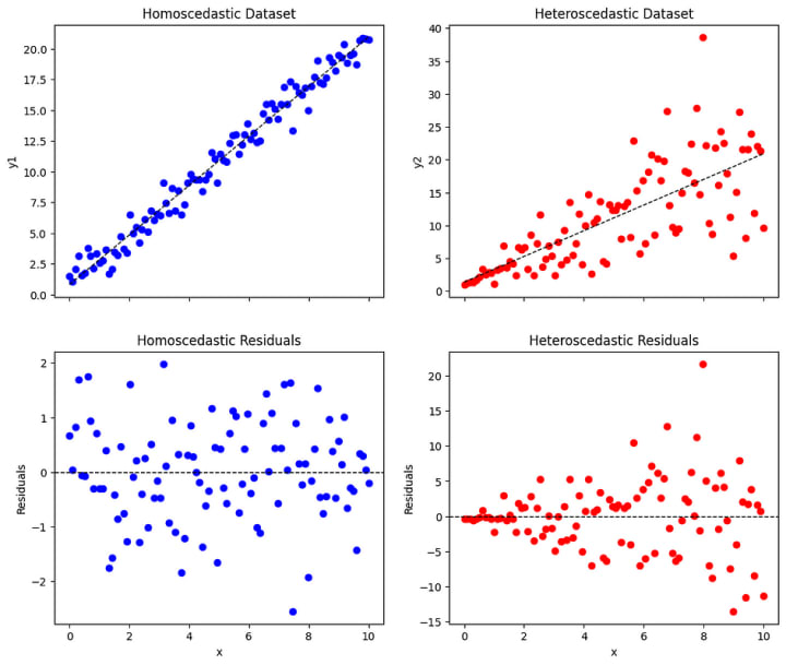
1. Residual plot: Create a scatter plot of the residuals (the differences between the observed and predicted values) against the predicted values or against each independent variable. If the plot shows a random scattering of points around zero with no discernible pattern, it suggests homoscedasticity. If there is a systematic pattern, such as a funnel shape or a curve, it indicates heteroscedasticity.
2. Breusch-Pagan test: This is a formal statistical test for heteroscedasticity. The null hypothesis is that the error variances are constant (homoscedastic). If the resulting pvalue is less than a chosen significance level (e.g., 0.05), the null hypothesis is rejected, indicating heteroscedasticity.

import numpy as np

import matplotlib.pyplot as plt

# Set random seed for reproducibility

np.random.seed(42)

# Generate data

x = np.linspace(0, 10, 100)

# Homoscedastic dataset

y1 = 2 * x + 1 + np.random.normal(0, 1, len(x))

# Heteroscedastic dataset

y2 = 2 * x + 1 + np.random.normal(0, x, len(x))

# Fit linear models

coeffs1 = np.polyfit(x, y1, 1)

y1_pred = np.polyval(coeffs1, x)

residuals1 = y1 - y1_pred

coeffs2 = np.polyfit(x, y2, 1)

y2_pred = np.polyval(coeffs2, x)

residuals2 = y2 - y2_pred

# Plot datasets and residuals

fig, axes = plt.subplots(2, 2, figsize=(12, 10), sharex=True)

# Plot dataset 1

axes[0, 0].scatter(x, y1, color='blue')

axes[0, 0].plot(x, y1_pred, color='black', linestyle='--', lw=1)

axes[0, 0].set_title('Homoscedastic Dataset')

axes[0, 0].set_ylabel('y1')

# Plot dataset 2

axes[0, 1].scatter(x, y2, color='red')

axes[0, 1].plot(x, y2_pred, color='black', linestyle='--', lw=1)

axes[0, 1].set_title('Heteroscedastic Dataset')

axes[0, 1].set_ylabel('y2')

# Plot residuals for dataset 1

axes[1, 0].scatter(x, residuals1, color='blue')

axes[1, 0].axhline(0, color='black', linestyle='--', lw=1)

axes[1, 0].set_title('Homoscedastic Residuals')

axes[1, 0].set_xlabel('x')

axes[1, 0].set_ylabel('Residuals')

# Plot residuals for dataset 2

axes[1, 1].scatter(x, residuals2, color='red')

axes[1, 1].axhline(0, color='black', linestyle='--', lw=1)

axes[1, 1].set_title('Heteroscedastic Residuals')

axes[1, 1].set_xlabel('x')

axes[1, 1].set_ylabel('Residuals')

plt.show()

What to do when the assumption fails?

1. Transformations: Apply transformations to the dependent and/or independent variables to stabilize the variance of the residuals. Common transformations include logarithmic, square root, and inverse transformations.
2. Weighted Least Squares (WLS): Use a weighted least squares approach, which assigns different weights to the observations based on the magnitude of their residuals. This method can help account for heteroscedasticity by giving more importance to observations with smaller residuals and less importance to those with larger residuals.
3. Robust standard errors: Calculate robust (or heteroscedasticity-consistent) standard errors for the regression coefficients. These standard errors are more reliable under heteroscedasticity and can be used to perform more accurate hypothesis tests and construct valid confidence intervals.

Breusch-Pagan Test

The Breusch-Pagan test, also known as the Cook-Weisberg test, is a statistical test used to detect heteroscedasticity in a linear regression model. The test is based on the assumption that the variance of the errors is a function of one or more independent variables. Here are the steps to perform the Breusch-Pagan test:

1. Estimate the linear regression model: Fit a linear regression model to the data using the ordinary least squares (OLS) method. Obtain the residuals (errors) from this model.
2. Calculate the squared residuals: Square each residual obtained in step1
3. Regress squared residuals on the independent variables: Perform another linear regression, this time with the squared residuals as the dependent variable and the same set of independent variables used in the original model. Obtain the R-squared value from this regression.
4. Calculate the test statistic: The Breusch-Pagan test statistic, known as the Lagrange Multiplier (LM) statistic, is calculated as follows: LM = n * R² where n is the number of observations and R² is the R-squared value obtained in step 3.
5. Determine the p-value: The LM statistic follows a chi-squared distribution with k degrees of freedom, where k is the number of independent variables (excluding the constant term). Calculate the p-value for the LM statistic using the chi-squared distribution.
6. Make a decision based on the p-value: Compare the calculated p-value to a chosen significance level (usually α = 0.05). If the p-value is less than or equal to α, reject the null hypothesis and conclude that there is evidence of heteroscedasticity in the data. If the p-value is greater than α, do not reject the null hypothesis and assume that the data exhibits homoscedasticity (constant variance of the residuals).

Note that the Breusch-Pagan test assumes a linear relationship between the independent variables and the variance of the errors. If the relationship is not linear, the test may not be appropriate, and other tests for heteroscedasticity should be considered.

# 4. No Autocorrelation

The Assumption

There should be no apparent correlation or pattern in the residuals, as this would suggest that the error terms are not independent.

What happens when this assumption is violated?

1. Inefficient estimates: The parameter estimates (coefficients) remain unbiased, but they are no longer the best linear unbiased estimators (BLUE). The inefficiency of the estimates implies that the standard errors may be larger than they should be, which may reduce the statistical power of hypothesis tests.
2. Inaccurate hypothesis tests: The t-tests and F-tests used to assess the significance of the regression coefficients and the overall model rely on the assumption of no autocorrelation. If the error terms exhibit autocorrelation, these tests may produce misleading results, leading to incorrect inferences about the significance of the independent variables.
3. Invalid confidence intervals: The confidence intervals for the regression coefficients are based on the assumption of no autocorrelation. If this assumption is violated, the confidence intervals may not be accurate, affecting the interpretation of the effect sizes and the precision of the estimates.

How to check this assumption

1. Durbin-Watson test: This is a formal statistical test for autocorrelation, specifically first-order autocorrelation. The Durbin-Watson test statistic ranges from 0 to 4, with a value of 2 indicating no autocorrelation. Values less than 2 suggest positive autocorrelation, while values greater than 2 indicate negative autocorrelation. It is important to note that the Durbin Watson test is only applicable for first-order autocorrelation and may not detect higher-order autocorrelation.

What to do when the assumption fails?

Lagged variables: Include lagged values of the dependent variable or the independent variables as predictors in the model to account for the autocorrelation.

Differencing: Apply differencing to the dependent and/or independent variables, which can help remove the autocorrelation by focusing on the changes between consecutive observations rather than the absolute values.

Generalized least squares (GLS): Use a generalized least squares approach that accounts for the autocorrelation structure in the error terms, leading to more efficient and reliable estimates.

Time series models: Consider using specialized time series models, such as autoregressive (AR), moving average (MA), autoregressive integrated moving average (ARIMA), or seasonal decomposition of time series (STL), which are designed to handle autocorrelation.

Robust standard errors: Calculate robust standard errors that are more reliable under autocorrelation, such as Newey-West standard errors or HAC (heteroscedasticity and autocorrelation consistent) standard errors.

Collab file link

# 5 No Multicollinearity

"Unpacking Multicollinearity: Understanding its Impact on Regression Analysis."

Multicollinearity is a statistical term used to describe a situation in which two or more independent variables in a…medium.com