
Content warning
This story may contain sensitive material or discuss topics that some readers may find distressing. Reader discretion is advised. The views and opinions expressed in this story are those of the author and do not necessarily reflect the official policy or position of Vocal.
"Mastering ROC AUC Curve: A Comprehensive Guide for Data Scientists"
"Unlocking the Power of ROC AUC Curve: A Practical Approach"
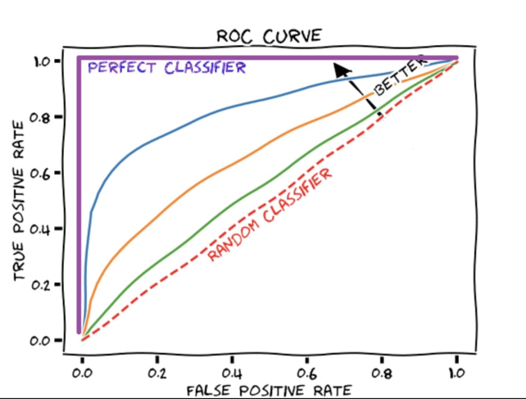
Why ROC Curve?
practical implementation after completing blog.
In supervised machine learning, we encounter two types of problems: regression and classification. In a regression problem, we aim to predict a numerical value, such as predicting the salary (LPA) based on features like CGPA and IQ. On the other hand, in a classification problem, we seek to predict the class or category to which a data point belongs. For example, determining whether a student is placed or not based on their CGPA and IQ.
When dealing with classification problems, especially binary classification, the ROC (Receiver Operating Characteristic) curve is widely used. The ROC curve helps us assess and visualize the performance of classification algorithms. In these algorithms, like logistic regression, the models calculate the probability (ranging from 0 to 1) of an event occurring, such as the likelihood of a student being placed.
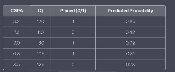
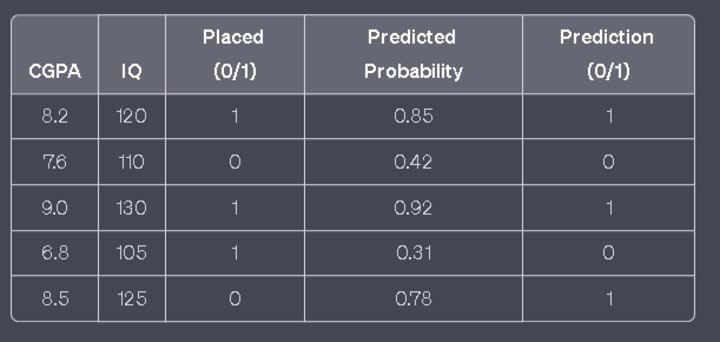
To convert predicted probabilities into actual predictions, we need to choose a threshold value. For instance, if the threshold is set to 0.5, any predicted probability below 0.5 is classified as 0 (not placed), while anything above 0.5 is classified as 1 (placed).
The question arises as to how we determine the optimal threshold value. This is where the ROC curve becomes crucial. It allows us to evaluate various threshold values and select the one that best suits our needs.
Let's consider another example of email classification. Suppose we want to predict whether an email is spam or not (threshold 0.5). There are two types of mistakes we can make:
False Negative: A spam email is incorrectly classified as not spam.
False Positive: A non-spam email is incorrectly classified as spam.
While the first case may result in inconvenience, such as seeing advertisements, we can manage the first case in case of email spam classifier problem it will not harm us to see ADS like myntra or something else
the second case is more problematic. For instance, imagine a college student receives an email about a job interview, but the model predicts it as spam with a probability of 0.6 (since 0.6 > 0.5). Consequently, the email ends up in the spam folder, and the student remains unaware of the interview opportunity. As a result, the student loses the interview and possibly the job. Such incidents can lead to a loss of trust in the predictive model.
-->Then the student will never use your product again
To avoid such errors, we need to determine the best threshold value. In this case, we could consider a higher threshold, such as 0.8, where probabilities above 0.8 are classified as spam. By fine-tuning the threshold, we can make more accurate predictions and minimize the chances of misclassifying important emails.
By utilizing the ROC curve and selecting an appropriate threshold value, we can enhance the performance and reliability of our classification models.
Confusion Matrix
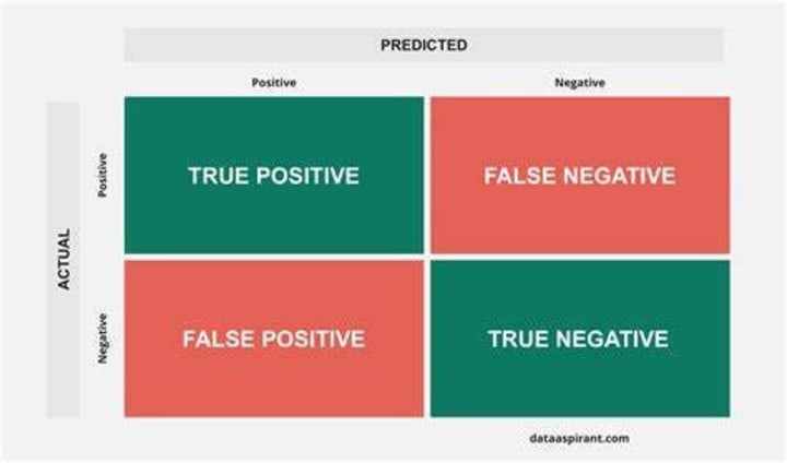
In email classification, the confusion matrix is a useful tool to evaluate the performance of a classification model. It provides a summary of the predictions made by the model compared to the actual labels. The matrix consists of four key metrics: true positives (TP), true negatives (TN), false positives (FP), and false negatives (FN).
Let's consider an example confusion matrix for an email classification model:

In this confusion matrix, we have the following metrics:
True Positives (TP): Emails that are actually spam and correctly predicted as spam. In this example, there are 85 true positives.
True Negatives (TN): Emails that are actually not spam and correctly predicted as not spam. Here, we have 92 true negatives.
False Positives (FP): Emails that are actually not spam but incorrectly predicted as spam. We have 8 false positives.
False Negatives (FN): Emails that are actually spam but incorrectly predicted as not spam. In this case, there are 15 false negatives.
In summary, the confusion matrix provides a comprehensive overview of the model's predictions and aids in evaluating its accuracy and performance in distinguishing between spam and non-spam emails.
True Positive Rate (TPR) -> Benefit
True Positive Rate (TPR), also known as sensitivity or recall, measures the proportion of correctly predicted positive cases out of all actual positive cases. In the context of email spam detection, TPR represents the ability of the model to correctly identify spam emails.
Let's consider an example to explain TPR in the context of email spam:
Suppose we have a dataset of 100 emails, out of which 40 are spam and 60 are not spam. After training our spam detection model, we obtain the following results:
True Positives (TP): 35 The model correctly identifies 35 spam emails as spam.
False Negatives (FN): 5 The model incorrectly classifies 5 spam emails as not spam.
True Negatives (TN): 55 The model correctly identifies 55 non-spam emails as not spam.
False Positives (FP): 5 The model incorrectly classifies 5 non-spam emails as spam.
Using these values, we can calculate the TPR as follows:
TPR = TP / (TP + FN) = 35 / (35 + 5) = 35 / 40 = 0.875 or 87.5%
The TPR of 87.5% indicates that our model correctly identified 87.5% of the actual spam emails in the dataset. In other words, it has a high sensitivity in detecting spam emails.
It is important to have a high TPR in spam detection to minimize the chances of missing important spam emails and to ensure a higher level of protection against potential threats. However, it is also crucial to consider other metrics, such as precision and specificity, to assess the overall performance of the spam detection system.
False Positive Rate (FPR)
False Positive Rate (FPR) measures the proportion of incorrectly predicted positive cases out of all actual negative cases. In the context of email spam detection, FPR represents the rate at which non-spam emails are incorrectly classified as spam.
Continuing with the previous example of email spam detection:
True Positives (TP): 35
False Negatives (FN): 5
True Negatives (TN): 55
False Positives (FP): 5
We can calculate the FPR as follows:
FPR = FP / (FP + TN) = 5 / (5 + 55) = 5 / 60 = 0.083 or 8.3%
The FPR of 8.3% indicates that 8.3% of the actual non-spam emails in the dataset were incorrectly classified as spam by the model. In other words, the model has a false positive rate of 8.3%.
A low FPR is desirable in email spam detection as it indicates a lower likelihood of legitimate emails being marked as spam. However, it's important to find a balance between minimizing false positives (non-spam emails classified as spam) and maximizing true positives (spam emails correctly classified as spam). Achieving a low FPR while maintaining a high TPR and precision is crucial for an effective spam detection system.
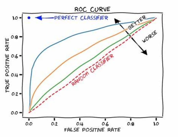
The Ultimate Goal
The ultimate goal in email spam detection is to achieve a high True Positive Rate (TPR) while maintaining a low False Positive Rate (FPR). By varying the threshold values used for classifying emails as spam or non-spam, we can plot a curve that shows the trade-off between TPR and FPR. This curve, often referred to as the Receiver Operating Characteristic (ROC) curve, provides a visual representation of the performance of the spam detection system at different classification thresholds. The goal is to find the optimal threshold that strikes a balance between identifying as many spam emails as possible (high TPR) and minimizing the number of legitimate emails classified as spam (low FPR). By analyzing the ROC curve and choosing an appropriate threshold, we can maximize the effectiveness of the spam detection system in accurately identifying spam emails while minimizing false positives.
coding implementation→ roc-auc.ipynb - Colaboratory (google.com)
About the Creator
Enjoyed the story? Support the Creator.
Subscribe for free to receive all their stories in your feed. You could also pledge your support or give them a one-off tip, letting them know you appreciate their work.
Keep reading
More stories from ajay mehta and writers in Education and other communities.
"Understanding Kurtosis and How to Determine if Your Data has a Normal Distribution."
What is Kurtosis? Kurtosis is a statistical term that measures the degree of peaked Ness or flatness of a distribution compared to the normal distribution. A distribution with high kurtosis has a sharp peak and fat tails, indicating that it has a higher probability of extreme values than a normal distribution. On the other hand, a distribution with low kurtosis has a flatter peak and thinner tails, indicating that it has a lower probability of extreme values than a normal distribution.
By ajay mehtaabout a year ago in Education
The Silent Guardians: Unveiling the Power of Your Kidneys
The Silent Guardians: Unveiling the Power of Your Kidneys Our bodies are marvels of intricate systems, working in perfect harmony to sustain life. While some organs, like the heart or lungs, garner more attention, others operate silently but no less critically. The kidneys, two unassuming bean-shaped organs nestled near your lower back, play a crucial role in maintaining our internal equilibrium – a state known as homeostasis. Understanding how these silent guardians function empowers us to adopt habits that promote their health and overall well-being.
By suren arju7 days ago in Education
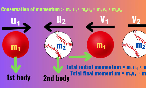
what is momentum class 9
Introduction: Physics is a fundamental science that seeks to explain the natural phenomena of the universe. Among its many interesting concepts momentum is one of them, which is a principle that plays a crucial role in the study of motion and dynamics. Momentum is a key concept that bridges the understanding of both motion and the forces that affect it. In this article, I will discuss into the concept of momentum,particularly what is momentum class 9 providing a thorough explanation with examples, equations, and real-life applications.
By champak jyoti7 days ago in Education


Comments
There are no comments for this story
Be the first to respond and start the conversation.