How to Forecast Time Series in Python?

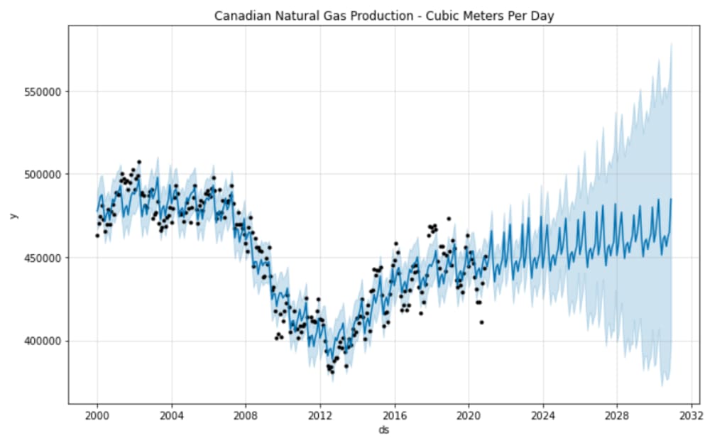
The idea of this post is to use a univariate time-series dataset provided by the Canadian Energy Regulator for natural gas production and produce a best-fit model that will allow us to predict future natural gas production for the next 10 years i.e. until 2030.

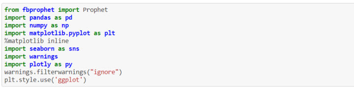
We will start by importing various libraries in Python such as fbprophet, numpy, pandas, seaborn, plotly and matplotlib. Please make sure you install these libraries before running the program. For your reference, the Jupyter notebook and CSV file have been uploaded my github page.

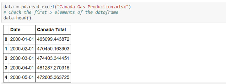
Next, we will import Canadian natural gas production data from Canada Energy regulator website, load that data into a pandas dataframe 'data'.

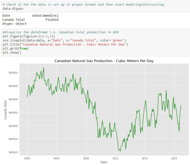
In the next step, we will check the data types and visualize the dataset using matplotlib library.

Prophet expects that the format of the dataframe to be specific. The model expects a ‘ds’ column that contains the datetime field and and a ‘y’ column that contains the value we are wanting to model/forecast.

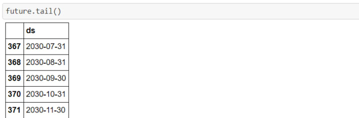
Now its time to start forecasting. With Prophet, we start by building some future time data with the following command:

In this line of code, we created a pandas dataframe with 120 (periods = 120) future data points with a monthly frequency (freq = ‘m’). In the next line of code, we check the last five dates of the forecasted data.

Now, we will try to predict the actual values using Prophet library and check the last five elements of the forecast.

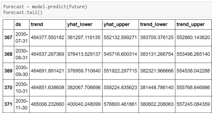
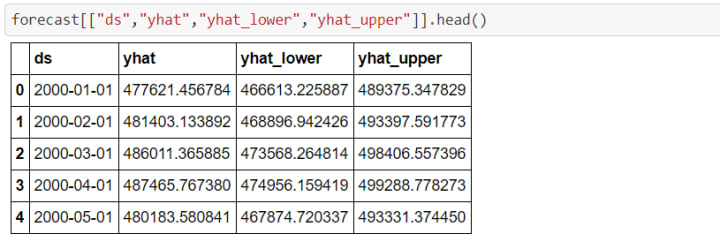
If we take a look at the data using .tail(), we notice there are a bunch of columns in the forecast dataframe. The important ones (for now) are ‘ds’ (datetime), ‘yhat’ (forecast), ‘yhat_lower’ and ‘yhat_upper’ (uncertainty levels).

Next, we will check the model robustness using the best metrics for measuring accuracy of this model. Utilizing a combination of R-Squared, Mean Squared Error and Mean Absolute Error will help us to gauge the quality of our model. We will Python's Scikit-Learn library to quickly calculate these metrics.

R-squared (R2) is a statistical measure that represents the proportion of the variance for a dependent variable that's explained by an independent variable or variables in a regression model.

Mean Absolute Error (MAE) measures the average magnitude of the errors in a set of predictions, without considering their direction. It’s the average over the test sample of the absolute differences between prediction and actual observation where all individual differences have equal weight.

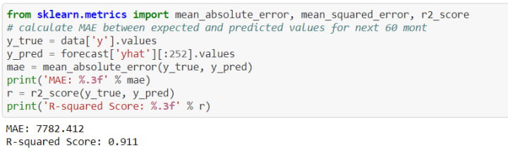
For the Canadian natural gas time-series data, the Prophet model gives an R-squared value of 0.91 i.e. 91% of variance in our data set is explained by the model. The MAE is calculated to be 7782 i.e. for each data point, the average magnitude error is roughly 7782 Cubic Meters Per Day, which isn't bad at all when we consider that our production value is in hundreds of thousands of Cubic Meters Per Day.

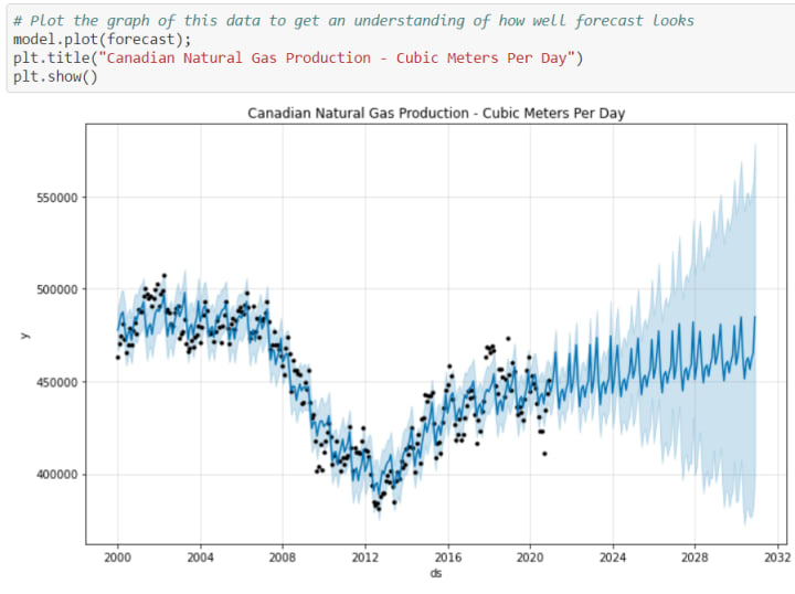
Finally, we create a plot to compare actual vs. predicted values to give a clear understanding of how our model visually looks against the existing Canadian natural gas production dataset.