Quora Question Pairs Similarity Problem

Quora is an American question-and-answer website where questions are asked, answered, followed, and edited by Internet users, either factually or in the form of opinions.

Over 100 million people visit Quora every month, so it’s no surprise that many people ask similarly worded questions. Multiple questions with the same intent can cause seekers to spend more time finding the best answer to their question and make writers feel they need to answer multiple versions of the same question. Quora follows canonical questions because they provide a better experience to active seekers and writers, and offer more value to both of these groups in the long term.

Business Problem

Identify which questions asked on Quora are duplications of questions that have already been asked.

This could be useful to instantly provide answers to questions that have already been answered. We are tasked with predicting whether a pair of questions are duplicates or not.

User Guide

The Colab Notebooks are available for this real-world use case at my GitHub repository!

Constraints

• The cost of misclassification can be very high.
• You would want a probability of a pair of duplicate questions so that you can choose any threshold of choice. Say, if you choose the probability threshold as 0.95 so Prob(Question 1 similar to Question 2) ≥0.95 then only merge the answers of Question 1 and 2 otherwise not.
• No strict latency concerns.
• Interpretability is partially important.

Understanding Data

You can download the dataset for the use case from Kaggle or my GitHub repository.

Data Overview

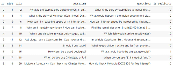
Data will be in a file train.csv. There are a total 404,290 number of observations or rows. It contains 6 columns: id(observation id), qid1 (first question id), qid2 (second question id), question1 (the textual content of the first question), question2 (the textual content of the second question), is_duplicate which is the label whether questions are duplicates or not denoted by 1 or 0 respectively.

Type of ML Problem

It is a binary classification problem, for a given pair of questions we need to predict if they are duplicates or not.

Exploratory Data Analysis

What is the total number of question pairs for training? — — 404,290.

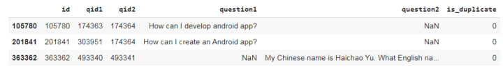
Are there any null or missing values in the data? — — question1 has 1 null object or missing value and question2 has 2 null objects or missing values. We will fill the missing values with blank strings.

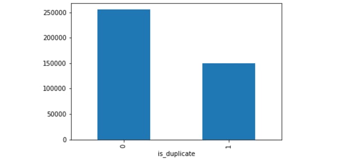
What is the distribution of final class labels?

The number of duplicates (similar or 1) questions is 149263 and the number of non-duplicate (non-similar or 0) questions is 255027 which constitute 36.92% and 63.08% of the data respectively. Only about 37% of the question pairs are similar!

How many are the unique questions? — — 537933

Illustration to find unique questions: In the below figure of dummy data, notice that the id of the question is repeating in the 4th and 5th row. The total number of observations is 5 but the unique number of questions is 6 which are 1,2,3,4,5 and 6. To find the unique number of questions, we should consider the number of unique question id’s from qid1 and qid2.

Around 21% of the unique questions are repeated more than once.

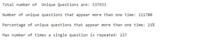
Which is the most repeating question? — — ‘What are the best ways to lose weight?’ is the question repeated 157 times. It seems people are more interested to know how to lose weight! :P

Are there any repeated pairs of questions? — — No!

Illustration to find whether any repeated pair of questions: In the below figure of dummy data, there 2 repeated pairs of questions, one with id 0 and 4 and the other with id 1 and 2.

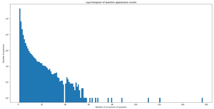
What is the number of occurrences for each question?

Note that the y-axis is the logarithmic axis, 10 power 0 is 1, and so on… Notice there is one question repeating around 160 times.

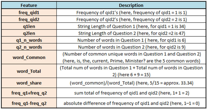
Feature Extraction Before Data Cleaning

Let us begin with feature engineering. We will extract 11 possible features, some of these features may be useful and some may not at all. After constructing the below features, we will have 17 columns in total including the output feature is_duplicate. Consider below dummy data for illustration:

Analysis of the features extracted above

• There are 67 questions in question 1 and 24 questions in question 2 with just one word!
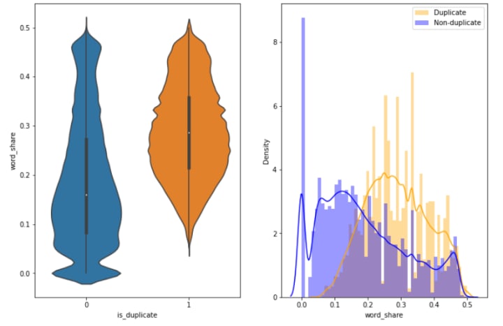
• The feature ‘word_share’ has quite a lot of predictive power, as it is good at separating the duplicate questions from the non-duplicate ones. The violin plot on the left shows that duplicate questions share more common words than non-duplicates hence word_share is higher for duplicates. The distributions for normalized word_share have some overlap on the far right-hand side, i.e., there are quite a lot of questions with high word similarity.
• Interestingly, it seems very good at identifying questions that are definitely different but is not so great at finding questions that are definitely duplicates.

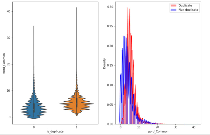
• In the below plot, the distributions of the word_Common feature in similar and non-similar questions are highly overlapping. Hence, this feature is not that useful to us.

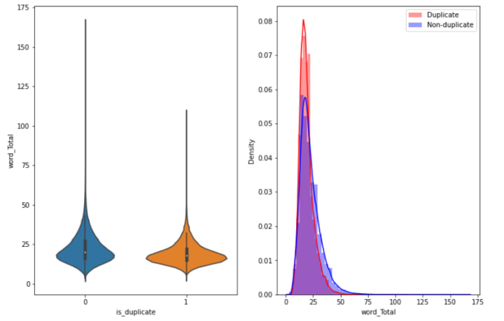
• In the below plot, the distributions of the feature word_Total are highly overlapping. Hence, this feature is not at all helpful in distinguishing duplicate and non-duplicate questions.

Semantic Analysis

Next, we will take a look at the usage of different punctuation in questions — this may form a basis for some interesting features later on.

• Questions with question marks: 99.87%
• Questions with [math] tags: 0.12%
• Questions with full stops: 6.31%
• Questions with capitalized first letters: 99.81%
• Questions with capital letters: 99.95%
• Questions with numbers: 11.83%

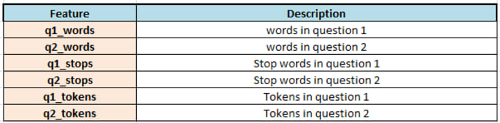
Advanced Feature Extraction (NLP and Fuzzy Features) After Data Cleaning

Consider ‘What is data science?’ sentence for illustration:

• Token: You get a token by splitting a sentence by a space.
• Ex.: ‘What’, ‘is’, ‘data’, ‘science?’ are the 4 tokens.
• Stop-Words: stop words as per NLTK.
• Ex.: here ‘is’ is the stop word.
• Word: A token that is not a stop_word.
• Ex.: ‘What’, ‘data’, ‘science?’ are the words.

Following are the 21 new features that we will extract:

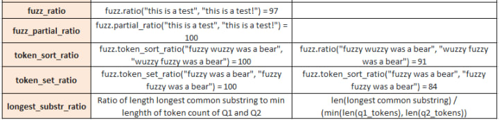
More information on fuzzy-wuzzy features.

Analysis of the features extracted above

• The number of data points or questions in class 1 (duplicate pairs): 298526
• The number of data points or questions in class 0 (non-duplicate pairs): 510054

After removing stop words from the questions:

• The total number of words in duplicate pair questions: 16109861
• The total number of words in non-duplicate pair questions: 33192952

Word clouds generated from duplicate pair question’s text:

donald trump, best way, 1k rupee are most occurring words in duplicate question pairs.

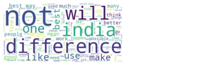
Word clouds generated from non-duplicate pair question’s text:

not, will, difference, India are the most occurring words in the non-duplicate question pairs.

T-SNE (t-distribution Stochastic Neighbourhood Embedding) for Visualization

T-SNE is the most used dimension reduction technique. It is a statistical method for visualizing high-dimensional data by giving each datapoint a location in a two or three-dimensional map.

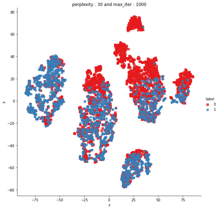
In the above 2-D graph, notice that there are few regions with maximum data points of only one class 0 (non-duplicates) or 1(duplicates) overlapped but there are few regions where you can quickly separate class region 0 or 1. Hence, this gives us a hint that the multiple dimensional features that we designed certainly have some value in differencing the two classes not perfectly but in some manner!

Featurization using TF-IDF weighted word2vec

We have noticed that some words occur more frequently in duplicate pairs of questions i.e., class 1 while some words occur more often in non-duplicate pairs of questions i.e., class 0 (refer to word clouds section).

• In this method, we will calculate the TF-IDF value of each word then sum the multiplication of the TF-IDF value with the corresponding word vector and divide this sum by the sum of the TF-IDF values.

Note that instead of word2vec, we will be using Glove (Global vectors).

• Both word2vec and Glove enable us to represent a word in the form of a vector (often called embedding). They are the two most popular algorithms for word embeddings that bring out the semantic similarity of words that capture different facets of a word's meaning. Word2vec embeddings are based on training a shallow feedforward neural network while glove embeddings are learned based on matrix factorization techniques.
• Word2Vec algorithms treat each word equally because of their goal to compute word embeddings. The distinction becomes important when one needs to work with sentences or document embeddings; not all words equally represent the meaning of a particular sentence. And here different weighting strategies are applied, TF-IDF is one of those successful strategies.
• At times, it does improve the quality of inference, so the combination is worth a shot.

Train and Test Split

The train-test split procedure is used to estimate machine learning algorithms performance when used to make predictions on data not used to train the model.

Think of temporal splitting or time-based splitting… assume your complete data is sorted by time and then you split the oldest data as train and the newest data as a test. Temporal splitting makes sense here as if the question asked is ‘Who is the current prime minister?’ then merging answers of the same question asked a few years back will give useless answers or results. As timestamp related feature is not available in the dataset so we cannot use the temporal splitting technique. Hence we build the train and test sets by randomly splitting in the ratio of 70:30 or 80:20 or whatever we choose as we have sufficient observations to work with!

Machine Learning Models

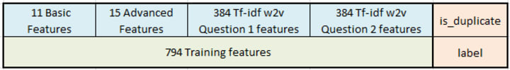
There is a total of 796 features in the dataset. The number of features in question1 w2v data frame and the number of features in question2 w2v data frame is the same i.e., 384. There is a total of 794 training features including the basic features extracted before data cleaning, the advanced NLP and fuzzy features extracted after data pre-processing, Tf-Idf vectors for question 1, and Tf-Idf vectors for question-2.

Here, we will split our data into train-test in the ratio of 70:30. The number of data points in train data: 283003 and the number of data points in test data: 121287. Let us call this test data, validation data because we already have test data that is completely unseen. You can download the test dataset from Kaggle.

What is log-loss?

Logarithmic Loss is the most important classification metric based on probabilities. It’s hard to interpret raw log-loss values, but log-loss is still a good metric for comparing models. Log loss is a metric that can lie between [0, infinity). For any given problem, a lower log-loss value means better predictions.

Log Loss is a slight twist on something called the Likelihood Function. In fact, Log Loss is -1 * the log of the likelihood function. So, we will start by understanding the likelihood function.

The likelihood function answers the question “How likely did the model think the actually observed set of outcomes was.” If that sounds confusing, an example should help.

For example, a model predicts probabilities [0.8, 0.4, 0.1] for three houses. The first two houses were sold, and the last one was not sold. So the actual outcomes could be represented numerically as [1, 1, 0].

Let’s step through these predictions one at a time to iteratively calculate the likelihood function.

The first house sold, and the model said that was 80% likely. So, the likelihood function after looking at one prediction is 0.8.

The second house sold, and the model said that was 40% likely. There is a rule of probability that the probability of multiple independent events is the product of their individual probabilities. So, we get the combined likelihood from the first two predictions by multiplying their associated probabilities. That is 0.8 * 0.4, which happens to be 0.32.

Now we get to our third prediction. That home did not sell. The model said it was 10% likely to sell. That means it was 90% likely to not sell. So, the observed outcome of not selling was 90% likely according to the model. So, we multiply the previous result of 0.32 by 0.9.

We could step through all of our predictions. Each time we’d find the probability associated with the outcome that actually occurred, and we’d multiply that by the previous result. That’s the likelihood!

Baseline Random Model

A baseline prediction algorithm provides a set of predictions that you can evaluate as you would any predictions for your problems, such as classification accuracy or loss. The random prediction algorithm predicts a random outcome as observed in the training data. It means that the random model predicts labels 0 or 1 randomly. The scores from these algorithms provide the required point of comparison when evaluating all other machine learning algorithms on your problem. More...

• The log loss on validation data using Random Model is 0.89. A lot of scope to reduce loss!

I have tried Logistic Regression as the data is fairly high dimensional and Linear SVM also. I have used SGDclassifier with ‘log’ loss which is actually a Logistic regression, and SGDclassifier with ‘hinge’ loss which is actually a Linear SVM and performed hyperparameter tuning on alpha(parameter of SGD classifier). But both the models didn’t gave promisible accuracy and hence log loss.

XGBoost Model

XGBoost is a decision-tree-based ensemble Machine Learning algorithm that uses a gradient boosting framework. The performance of XGBoost is no joke — it’s become the go-to library for winning many Kaggle competitions. More…

After fitting XGBoost Model on the training data, following are the results:

• The log loss on train data is 0.69 and on validation data is also approx. 0.69. Log loss reduced much better but again much scope for improvement!
• After applying some hyperparameter tunning, at the end achieved the log loss for training data is 0.345 and for validation is 0.357 which is a significant improvement.
• Also both the losses are close shows that model is neither over-fitting not under-fitting.

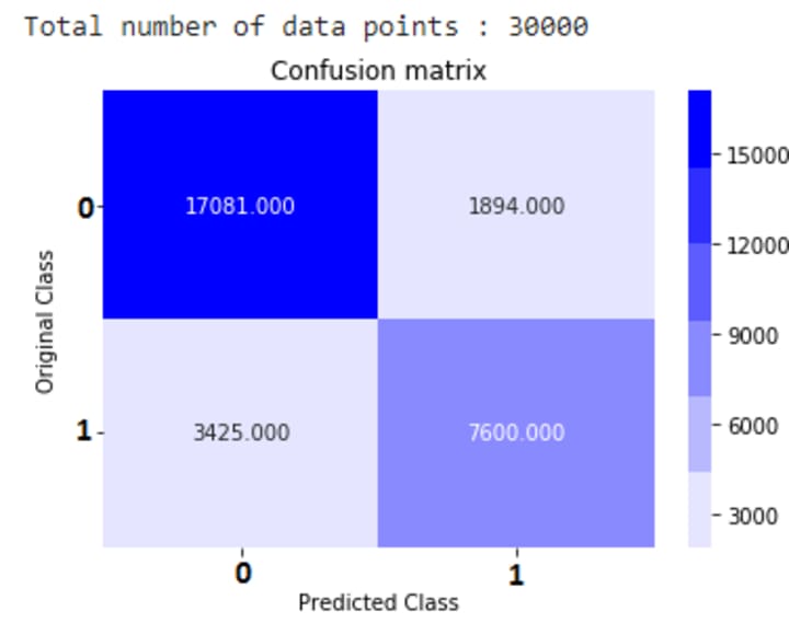
The true positives (17081) and true negatives(7600) are in large numbers which shows larger number of correct classifications. Check here for evaluation metrics used for classification problems and their interpretations.

• The precision for class 0 is 83% and for class 1 is 80%.
• Also, the recall for class 0 is 90% and for class 1 is 69%.
• Both are significant improvements over the above two linear models, logistic regression and linear SVM.

Now the task for you to apply the same pre-processing steps for test data and apply the above-trained model for the predictions!

__________________________________________

Thanks for reading ❤.

If you liked the article, please share it, so that others can read it!

Happy Learning! 😊