Pyomo for Solving Linear Programming Problems

This is a beginner-friendly introductory tutorial on Pyomo. Pyomo stands for Python Optimization Modeling Objects. In this tutorial, we learn how to solve linear programming problems (LPPs) using Pyomo which is an algebraic modeling language. It is a Python-based, open-source optimization modeling language. Although Pyomo has a diverse set of optimization capabilities, in this tutorial, we will discuss how to solve LPPs using Pyomo.

In this tutorial, we assume that the readers have basic knowledge of the Python programming language, and they are acquainted with the LPPs. Here, we consider an optimization problem and then we formulate it as a linear programming problem (LPP). After that, we learn how to write a Pyomo-based model using Python to solve the problem.

To know more about the author of this tutorial, please visit the link below.

An optimization problem from a chocolate manufacturing company

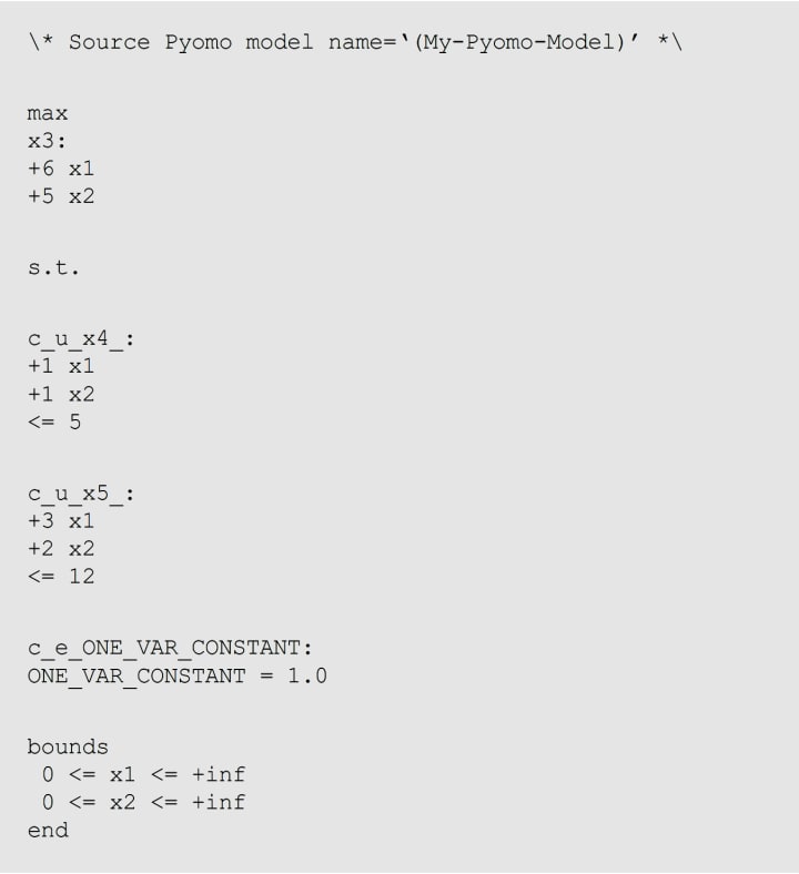
Consider a chocolate manufacturing company that produces only two types of chocolate — A and B. Both the chocolates require Milk and Choco only. To manufacture each unit of A and B, the following quantities are required:

• Each unit of A requires 1 unit of Milk and 3 units of Choco,
• Each unit of B requires 1 unit of Milk and 2 units of Choco.

The company kitchen has a total of 5 units of Milk and 12 units of Choco. On each sale, the company makes a profit of

• Rs. 6 per unit A sold,
• Rs. 5 per unit B sold.

Now, the company wishes to maximize its profit. How many units of A and B should it produce, respectively?

To read more tutorials from the author, please visit the link below.

Mathematical formulation

Now, we formulate the above optimization problem as an LPP. An LPP has mainly three components — decision variables, the objective function, and constraints.

Decision variables:

• x be the total number of units produced by A,
• y be the total number of units produced by B.

Objective function:

Maximize 6x + 5y

Constraints:

x + y ≤ 5

3x + 2y ≤ 12

x ≥ 0

y ≥ 0

The last two constraints are known as the non-negativity constraints.

Installing Pyomo

We assume that Python is already installed on your system before installing Pyomo. We can use both pip and conda commands to install Pyomo on our system.

We can use the following pip command to install Pyomo:

pip install pyomo

We can also use the conda command to install Pyomo as follows:

conda install -c conda-forge pyomo

Note that Pyomo does not include any stand-alone optimization solvers. Therefore, we need to install third-party solvers such as CBC, CPLEX, etc. to solve optimization models built with Pyomo.

In this tutorial, we use the CPLEX solver to solve the optimization model. Hence, we also assume that the IBM ILOG CPLEX Optimization Studio is already installed. If you are not sure how to install CPLEX, you can consult the tutorial from this link.

Pyomo model

Here, we write down the Pyomo model for the example problem mentioned above. At first, we import the required packages.

Import required packages

Create a model

Now, we are ready to create a Pyomo model. We can use the following command to create a model:

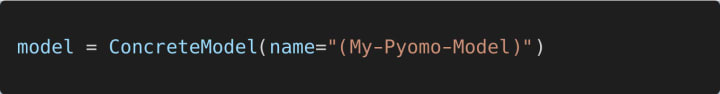
A concrete Pyomo model is created using the above command. Note that the argument 'name' is optional.

Define decision variables of the model

As discussed in the above mathematical problem formulation, we have two decision variables. These two decision variables can be defined as follows:

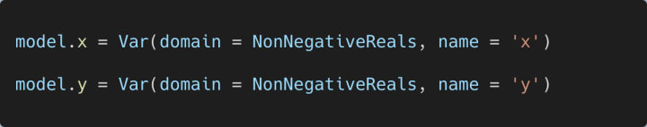
Here, we have set the domains of both the decision variables as non-negative reals, i.e., x ≥ 0 and y ≥ 0.

Define the objective function of the model

Now, the task is to define the objective function of the model. This can be done using the following command:

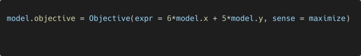
In the above command, we have passed the value 'maximize' to the argument 'sense' because the current problem described above is a maximization problem. For the minimization problem, this argument should be set as 'minimize'.

Add constraints to the model

We now add constraints to the model as defined above in the mathematical problem definition. Here, we have two constraints. These can be added to the model as follows:

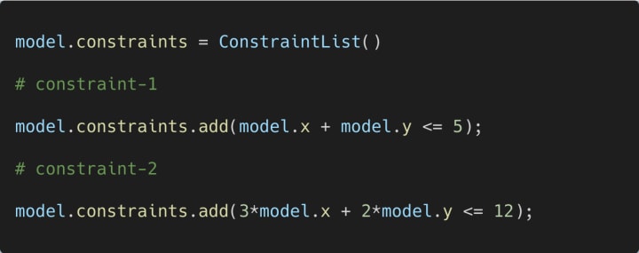
Note that we can use a semicolon at the end of each command used to define a constraint. This will suppress unnecessary output.

We can also note that we don’t need to include the non-negativity constraints (x ≥ 0, y ≥ 0) because, by default, these are already included in the definition of the decision variables.

Create a solver

Now, we create a solver. As mentioned above here we use the CPLEX solver. The following command can be used to create a solver:

Here, we have used IBM's CPLEX solver. We can use other solvers too. Note that we may need to specify the absolute solver path if it is not available as a system PATH variable. In the above command, we have used the absolute path of the solver (in this case, the solver is IBM's CPLEX).

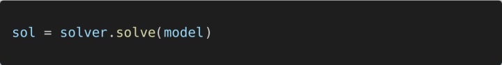
Solve the model

Now, we need to invoke the solver to start the optimization process. This can be done using the following command:

Print the solution

The solver will take some time to solve the optimization problem that we have just modeled above. At the end of the execution, it will produce some results. We can show these results by printing the solution. This can be done as follows:

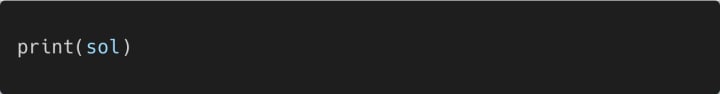
The above print statement will show relevant information regarding the solution.

Retrieving decision variables' values

We can easily retrieve the decision variables' values. This can be done using the following commands:

The outputs of the above print statements are shown below:

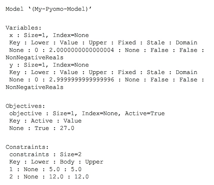
x = 2.0000000000000004

y = 2.9999999999999996

Retrieve the objective value

The objective function value can also be retrieved from the obtained solution, as follows:

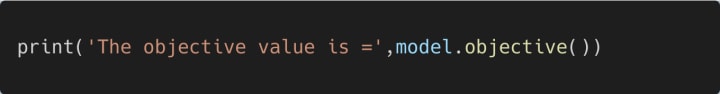
The output of the above print statement is:

The objective value is = 27.0

Save the model in a file

We can also save the model in a .lp file as follows:

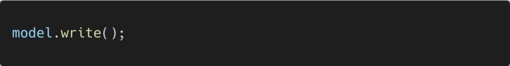
The above command will create a file named ‘(My-Pyomo-Model)’.lp. The contents of this file are shown below:

Display model information

Additionally, we can also view the information of the created model, as follows:

The above command will create a file named ‘(My-Pyomo-Model)’.lp. The contents of this file are shown below:

This is the end of this tutorial. In this tutorial, we have learned how to write a mathematical optimization model using Pyomo, and then solve it using IBM's CPLEX solver. To read interesting tutorials, you can subscribe to me.

Subscribe to the YouTube channel of Dr. Soumen Atta, Ph.D.