Machine Learning Model Performance Metrics

The idea of building machine learning models works on a constructive feedback principle. You build a model, get feedback from metrics, make improvements and continue until you achieve a desirable accuracy. Performance metrics as the name suggests explaining the performance of a model. An important aspect of performance metrics is their capability to discriminate among model results.

I have seen plenty of analysts and aspiring data scientists not even bothering to check how robust their model is. Once they are finished building a model, they hurriedly map predicted values on unseen data. This is an incorrect approach.

A model is considered to be robust if its output dependent variable (label) is consistently accurate even if one or more of the input independent variables (features) or assumptions are drastically changed due to unforeseen circumstances. Simply building a predictive model is not your motive. It’s about creating and selecting a model which gives high accuracy on out-of-sample data. Hence, it is crucial to check the accuracy of your model prior to computing predicted values.

There are different kinds of metrics to evaluate our models. After you are finished building your model, these 6 metrics will help you in evaluating your model’s accuracy.

Contents

1. Quick Warm-up: Types of Predictive model
2. Illustration with example
3. Confusion Matrix
4. Classification Accuracy
5. Precision
6. Recall
7. F1-Score
8. AUC-ROC

Quick Warm-up: Types of Predictive models

When we talk about predictive models, we are talking either about a regression model (continuous output) or a classification model (nominal or binary output). The evaluation metrics used in each of these models are different. In classification problems, we use two types of algorithms (dependent on the kind of output it creates):

• Class output: Algorithms like SVM and KNN create a class output. For instance, in a binary classification problem, the outputs will be either 0 or 1. However, today we have algorithms that can convert these class outputs to probability. But these algorithms are not well accepted by the statistics community.

• Probability output: Algorithms like Logistic Regression, Random Forest, Gradient Boosting, Adaboost, etc. give probability outputs. Converting probability outputs to class output is just a matter of creating a threshold probability.

In regression problems, we do not have such inconsistencies in output. The output is always continuous in nature and requires no further treatment.

Illustration with example

For a classification model evaluation metric discussion, I have used my predictions for one of the binary classification problems on Kaggle. The solution to the problem is out of the scope of our discussion here. However, the final predictions on the training set have been used for this article for illustration. The predictions made for this problem were probability outputs which have been converted to class outputs assuming a threshold of 0.5.

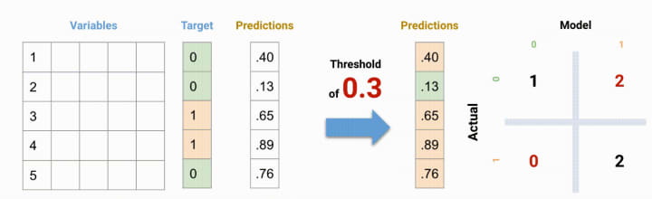
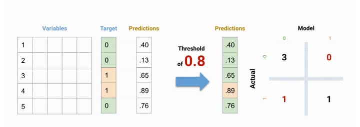
See in the above, there are 5 input samples in the data out of which 3 belongs to Negative (class 1) and 2 belongs to Positive (class 0). Considering the threshold of 0.5, the 5th observation with a probability of 0.76 is misclassified to class 1.

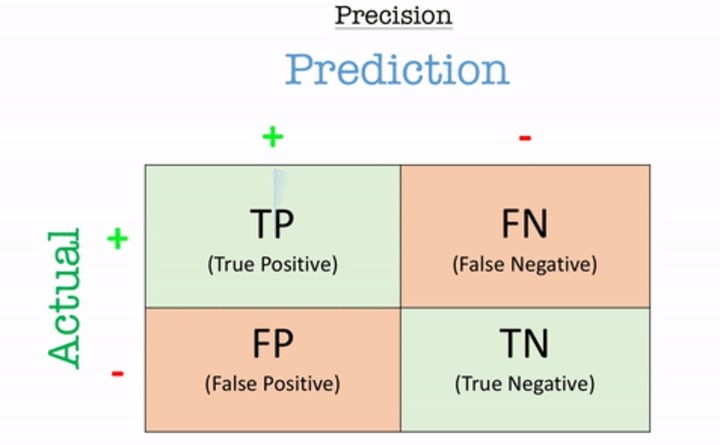
Confusion Matrix

A confusion matrix is an N X N matrix, where N is the number of classes being predicted. In the above example, we have N=2, and hence we get a 2 X 2 matrix.

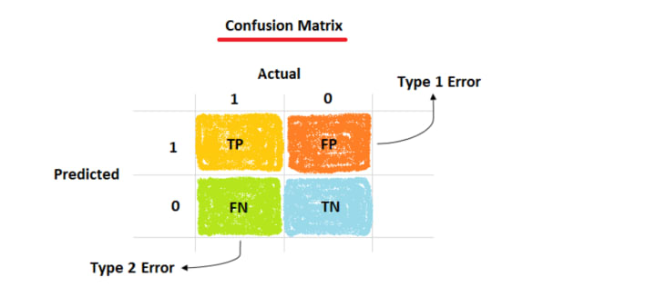
There are 6 important terms :

• True Positives: The cases in which we predicted Positive and the actual output was also Positive. Here, true positives are 2.
• True Negatives: The cases in which we predicted Negative and the actual output was Negative. Here, true negatives are 2.
• False Negatives: The cases in which we predicted Negative and the actual output was Positive. I remember it as falsely predicting Negative. Here, false negatives are 1.
• False Positives: The cases in which we predicted Positive and the actual output was Negative. I remember it as falsely predicting Positive. Here, No false positives i.e., 0.

• Type I Error: In statistical hypothesis testing, is the error caused by rejecting a null hypothesis when it is true. It is caused when the hypothesis that should have been accepted is rejected. It is denoted by α (alpha) known as an error, also called the level of significance of the test.
• Type II Error: It is the error that occurs when the null hypothesis is accepted when it is not true. In simple words, it means accepting the hypothesis when it should not have been accepted. It is denoted by β (beta) and is also termed as the beta error.

Classification Accuracy

Classification Accuracy is what we usually mean when we use the term accuracy.

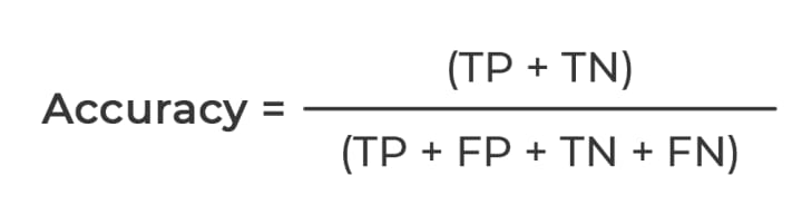
Accuracy is the ratio of the number of correct predictions to the total number of input samples or observations. Informally, accuracy is the fraction of predictions our model got right.

Here, Accuracy = (2+2)/(2+0+1+2) = 4/5 ie., 80%.

For example, consider that there are 98% samples of class 0 and 2% samples of class 1 in our training set. Then our model can easily get 98% training accuracy by simply predicting every training sample belonging to class 0.

When the same model is tested on a test set with 60% samples of class 0 and 40% samples of class 1, then the test accuracy would drop down to 60%. Classification Accuracy is great but gives us the false sense of achieving high accuracy.

The real problem arises when the cost of misclassification of the minor class samples is very high. If we deal with a rare but fatal disease, the cost of failing to diagnose the disease of a sick person is much higher than the cost of sending a healthy person to more tests.

Precision

Precision is the number of correct positive results divided by the number of positive results predicted by the classifier. The result is a value between 0.0 for no precision and 1.0 for full or perfect precision. Precision looks to see how much junk positives got thrown in the mix. If there are no bad positives (those FPs), then the model had 100% precision.

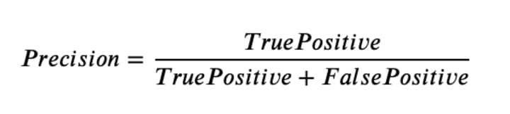
Here, Precision = 2/(2+0) = 1 ie., 100%.

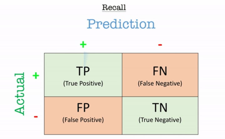
Recall

Recall is the number of correct positive results divided by the number of all relevant samples (all samples that should have been identified as positive). The result is a value between 0.0 for no recall and 1.0 for full or perfect recall.

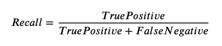
Here, Recall = 2/(2+1) = 2/3 i.e., 67%

Unlike precision that only comments on the correct positive predictions out of all positive predictions, recall provides an indication of missed positive predictions.

F1-Score

The harmonic mean of Precision and Recall. It is a single score that represents both Precision and Recall.

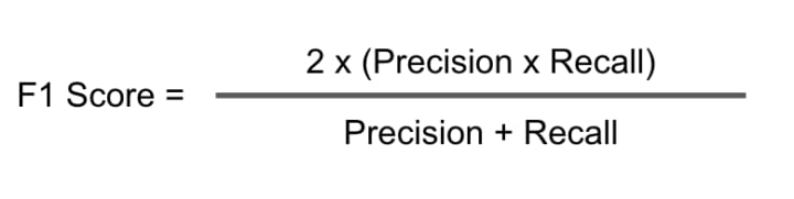
Here, F1-score = (2*1*0.67)/(1+0.67) = 0.80 .

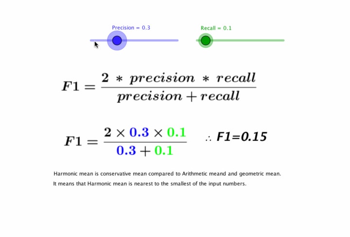
So why Harmonic Mean, why not Arithmetic Mean? Because it punishes extreme values more.

Consider a trivial method (e.g. always returning class 0). There are infinite data elements of class 1 and a single element of class 0:

Precision = 0.0 and Recall = 1.0

When taking the arithmetic mean, it would have 50% correct. Despite being the worst possible outcome! But, with the harmonic mean, the F1-score is 0.

Arithmetic mean = 0.5 and Harmonic mean = 0.0

In other words, to have a high F1-Score, you need to have both high precision and recall.

AUC-ROC (Area Under Curve - Receivers's Operating Curve)

Area Under Curve(AUC) is one of the most widely used metrics for evaluation. It is used for binary classification problems. AUC of a classifier is equal to the probability that the classifier will rank a randomly chosen positive example higher than a randomly chosen negative example. A ROC curve is a graph showing the performance of a classification model at all classification thresholds.

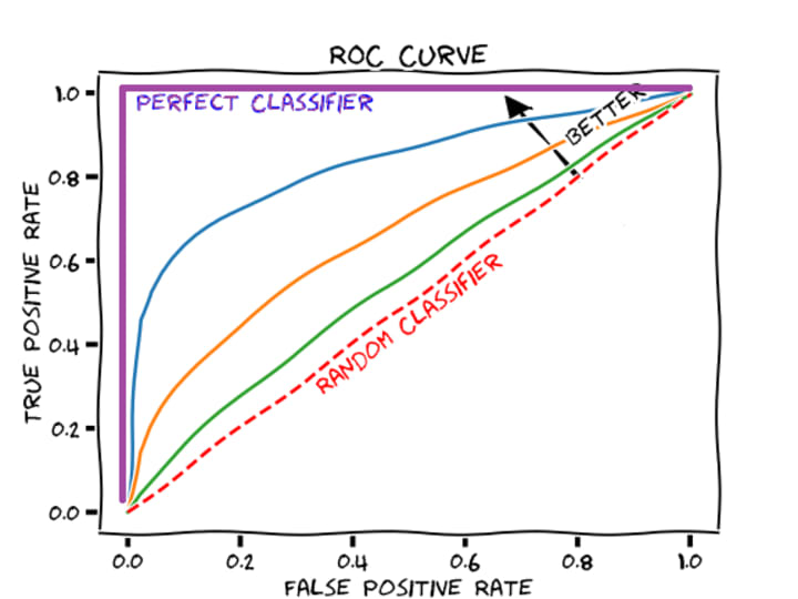
Axes for ROC are TPR (True Positive Rate) and FPR (False Positive Rate).

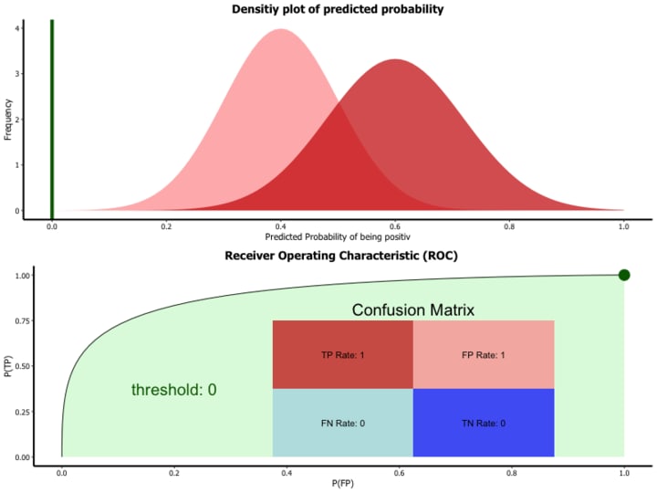
• True Positive Rate TPR (Sensitivity): True Positive Rate is defined as TP/ (FN+TP). True Positive Rate corresponds to the proportion of positive data points that are correctly considered as positive, with respect to all positive data points.

• True Negative Rate TNR (Specificity): True Negative Rate is defined as TN / (FP+TN). False Positive Rate corresponds to the proportion of negative data points that are correctly considered as negative, with respect to all negative data points.

• False Positive Rate FPR: False Positive Rate is defined as FP / (FP+TN). False Positive Rate corresponds to the proportion of negative data points that are mistakenly considered as positive, with respect to all negative data points.

False Positive Rate and True Positive Rate both have values in the range [0, 1]. FPR and TPR both are computed at varying threshold values such as (0.00, 0.02, 0.04, …., 1.00) and a graph is drawn.

AUC is the area under the curve of plot False Positive Rate vs True Positive Rate at different points in [0, 1]. As evident, AUC has a range of [0, 1]. The greater the value, the better is the performance of our model. The curve tells us how well the model can distinguish between the two classes. Better models can accurately distinguish between the two. Whereas, a poor model will have difficulties distinguishing between the two.

That’s it!

Thanks for reading ❤.

If you liked the article, please share it, so that others can read it!

Happy Learning!😊