Understand How Item Based Collaborative Filtering Works

Recommendation systems have been around us for quite some time now. Youtube, Facebook, Amazon, and many others provide some sort of recommendations to their users. This not only helps them show relevant products to users but also allows them to stand out in front of competitors.

One such technique to recommend items to users is an item-based recommendation system also known as item-item collaborative filtering or IBCF. In this guide, we will go through all the ins and outs of the algorithm, the actual mathematics behind it then will implement it in R, first without using any libraries, this will help understand how the algorithm fits in with the dataset, and then implement same using recommenderlab, an R package, to show how things work in a real environment.

ITEM — ITEM Collaborative Filtering

Item-item collaborative filtering is one kind of recommendation method which looks for similar items based on the items users have already liked or positively interacted with. It was developed by Amazon in 1998 and plays a great role in Amazon’s success.

How IBCF works is that it suggests an item based on items the user has previously consumed. It looks for the items the user has consumed then it finds other items similar to consumed items and recommends accordingly.

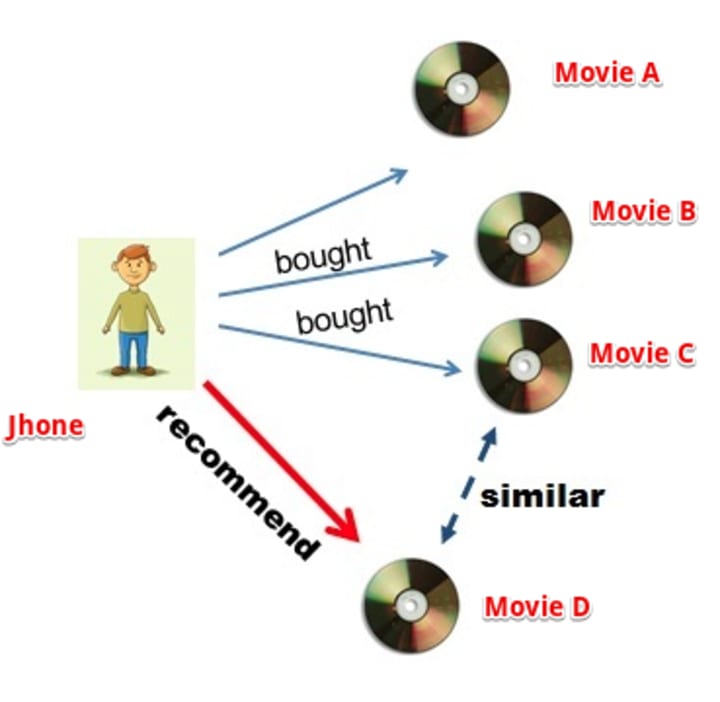
Let’s understand this with an example. Suppose our user Jhone wants to purchase a movie DVD. Our job is to recommend him a movie based on his past preferences. We will first search for movies that Jhone has watched or liked, let’s call those movies ‘A’, ‘B’ and ‘C’. Next, we will search for other movies similar to three movies. Suppose we found out that movie ‘D’ is highly similar to ‘C’, therefore, there is a highly likely chance that Jhone will also like movie ‘D’ because it is similar to one Jhone has already liked. Hence, we will suggest the movie ‘D’ to Jhone.

So at its core IBCF is all about finding items similar to the ones user has already liked. But how to find similar items? and what if there are multiple similar items in that case which item to suggest first? To understand this lets’ first understand the intuition behind the process, this will assist us to comprehend the mathematics behind the IBCF recommendation filtering.

If you want to dig deeper into item-based filtering I suggest starting with this course here. Mentors not only explain all the ins and outs of the algorithms but also explains its applications with real-world examples which is valuable for anyone who wants to advance in the recommender systems field.

Finding Similarity Between Items

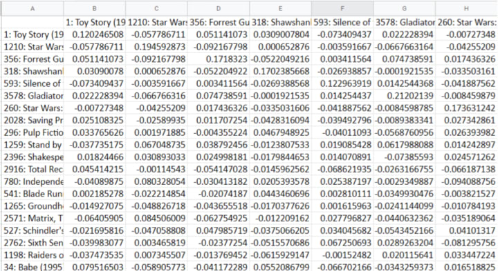
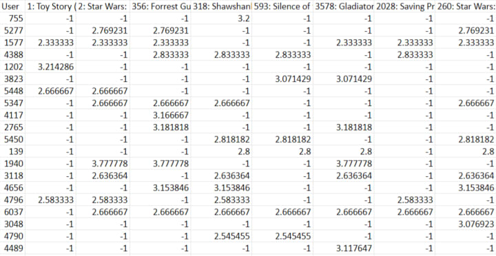
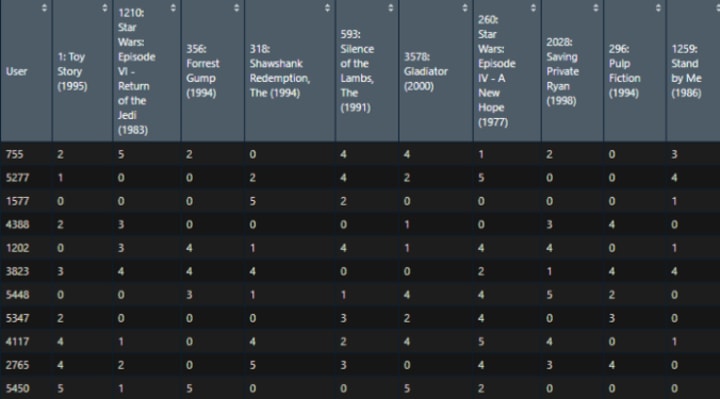
Suppose we have a table of users and their ratings for movies (link):

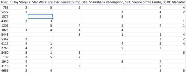
Let’s pick two movies (Id 1: Toy Story and Id 2: Star Wars) for which we have to calculate the similarity i.e. how much these two movies are comparable to one another in terms of their likeness by users. To compute this we will:

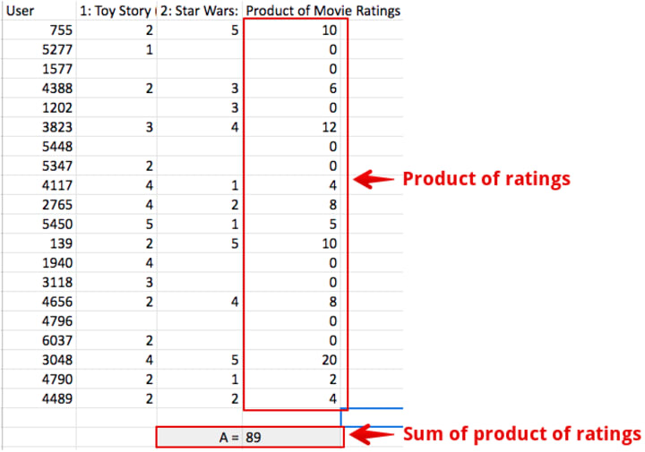
First multiple ratings of both the movies with each other and the sum the result. Let’s call this value ‘A’.

Second, we‘ll sum the squared movie ratings and then take the square root of them. So square all movie 1 ratings, sum them and then take the square root to get final value (do same of movie 2). Doing so will get us two values i.e. square root value of movie 1 and movie 2. Multiply both the values. We call this final value ‘B’.

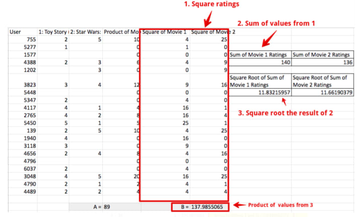
Third, divide A and B, this will gets us a score that indicates how close movie 1 and movie 2 are to one another (link).

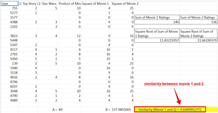
Repeating the above process for all the movies will result in a table with similarities between each movie(in general we call them items).

Here is how the above process is depicted in mathematical form.

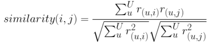
Don’t get overwhelmed by how crazy the formula looks. It‘s really simple and is exactly what we did above with our excel exercise. Let’s break it down piece by piece to understand what all these weird symbols mean.

Adding some labels to the letters will ease in understanding each part of the equation.

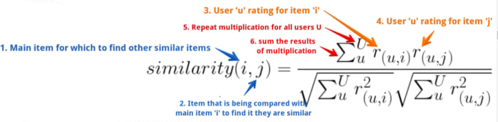
Starting from label 1 (blue on left), above illustrates that in order to calculate the similarity between an item ‘i’ and an item ‘j’ (consider ‘i’ and ‘j’ as movie id 1 and 2) multiple all ratings of item ‘i’ and ‘j’ given by users ‘u’ and sum them. Divided the result with the product of square root of the sum of squared ratings of individual items given by user ‘u’.

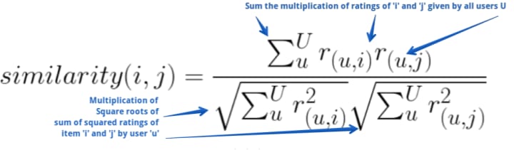
This is exactly what we did in our excel exercise above. Iterating above for all the items will result in a list of values that will indicate how close other items are to our main item ‘i’. This method is also known as cosine similarity. It helps to calculate how close two vectors are to one another.

Optimistic Nature of Users

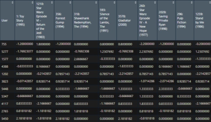
Cosine similarity works but it doesn’t take into account the optimistic behavior of users. Different users can rate the same item differently depending upon how optimistic they are. On a scale of 5, one could rate an item 5 while another could rate 3 even though they both very much liked the item. To account for this we have to make a small change to our similarity formula. Here is what it looks like.

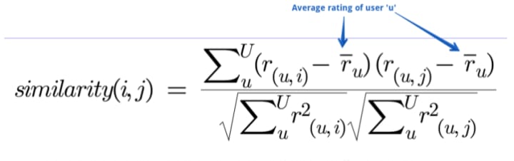
Subtracting user rating of a given item with that user’s average rating normalizes ratings to the same scale and helps overcome optimism issues. We call it adjusted cosine similarity.

There is also a similar method where instead of subtracting with the user’s average rating we subtract with items average rating. This helps to understand how much given user ratings deviate from average item rating. This technique is known as Pearson similarity. Both Cosine and Pearson are widely used methods to compute similarities.

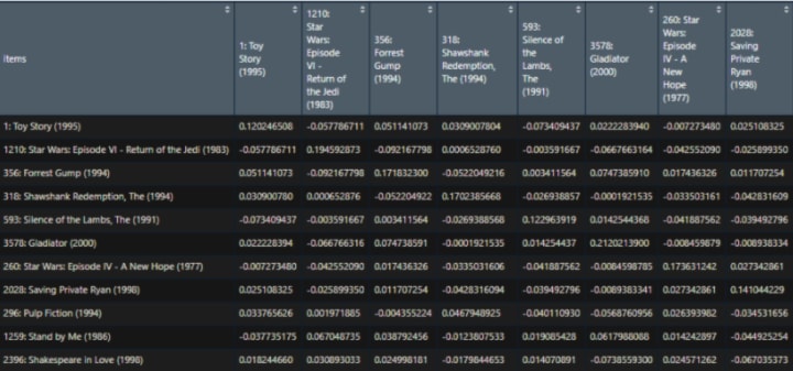
Applying adjusted cosine similarity equation on ratings for items will produce a table or matrix that’ll show how similar one item is to another. It should look something like this:

Calculate Recommendation Score

A table of similar items is a half job done. We know which items are comparable but we have yet to crack the nut on which items to recommend to users from the list of similar items. For this will have to combine our similarity matrix with users' past history of rated items to generate a recommendation. This is easily achieved by applying IBCF’s equation.

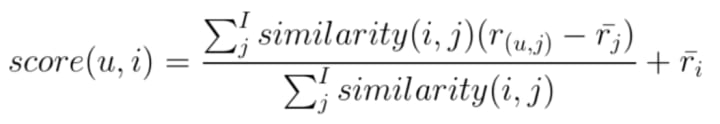
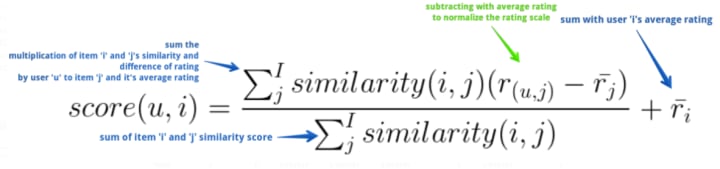
u = user for which we are generating recommendation

i = item in consideration, i.e. if this item should be recommended or not

score(u,i) = generates a score that will indicate how strong a recommendation of item ‘i’ is to our user ‘u’.

j = items similar to main item i.

Above equation elicits that in order to calculate recommendation score of an item ‘i’ for a user ‘u’ sum the multiplication of an item ‘i’ and ‘j’ similarity with the difference of rating given by user ‘u’ to an item ‘j’ and the average rating of an item ‘j’. Divide the result with the sum of item ‘i’ and ‘j’s similarity, add the output with the user ‘u’s average rating.

Doing so will generate a matrix of scores for users and available items. Top scored items can be recommended to the user.

IBCF Implementation Using R

Let’s see above in action using R (code link). This will allow us to further our understanding of IBCF.

Note: We will be using loops and data frames to implement IBCF knowing that R is fairly slow with loops and row/column multiplication is faster with matrix than with data frames. The reason being that the main purpose of this exercise is to help understand how IBCF is implemented using programming and we are not interested in writing robust code. Will show a faster alternative in section three of this article.

With that said let’s start by loading required libraries and movie rating data set.

library(dplyr)

##movie rating data

library(readxl)

data <- read_excel("C:/Users/muffaddal.qutbuddin/IBCF/movie rating.xlsx")

## replace na with zero

data[is.na(data)] <- 0

#view rating data set

View(data)

To calculate IBCF based on movie ratings, first, we will calculate normalize ratings by subtracting item ratings with user’s average rating. This will standardize ratings to the same scale.

## create a copy of rating dataframe

data.normalized<-data[FALSE,]

##normalize user rating

for (u in 1:nrow(data)) {

#get rating of the user for each item

ratings <-as.numeric(data[u,-1])

#calculate average rating

meanAvg <- mean(ratings[ratings!=0])

#iterate each user ratings.

# we start with 2nd column as first column is user id

for (j in 2:ncol(data)) {

#store user id in normalized dataframe

data.normalized[u,1]<-data[u,1]

#store zero incase of no rating

if(data[u,j]==0){

data.normalized[u,j] <- 0

}

#subtract user's item rating with average rating.

else{

data.normalized[u,j] <- data[u,j] - meanAvg

}

}

}

#view normalized ratings

View(data.normalized)

Next, we’ll calculate the similarity of each item by passing the actual rating and normalized rating to our ‘calCosine’ function.

data.ibs<-data[,-1]

data.normalize.ibs<-data.normalized[,-1]

data[data=0] <- NA

#function to calculate cosine similarity

calCosine <- function(r_i_normalized,r_j_normalized,r_i,r_j)

{

return(sum(r_i_normalized*r_j_normalized) / (sqrt(sum(r_i*r_i)) * sqrt(sum(r_j*r_j))))

}

#create an emptry table to store similarity

data.ibs.similarity <- read.table(text = "",

colClasses = rep(c('numeric'),ncol(data.normalize.ibs)),

col.names = c('items',colnames(data.normalize.ibs)),

check.names=FALSE)

# Lets fill in those empty spaces with cosine similarities

# Loop through the columns

for(i in 1:ncol(data.normalize.ibs)) {

# Loop through the columns for each column

for(j in 1:ncol(data.normalize.ibs)) {

#get movie name for which to calculate similartiy

data.ibs.similarity[i,1] <- colnames(data.normalize.ibs)[i]

# Fill in cosine similarities

data.ibs.similarity[i,j+1] <- calCosine(as.matrix(data.normalize.ibs[,i]),as.matrix(data.normalize.ibs[,j]),as.matrix(data.ibs[,i]),as.matrix(data.ibs[,j]))

}

}

View(data.ibs.similarity)

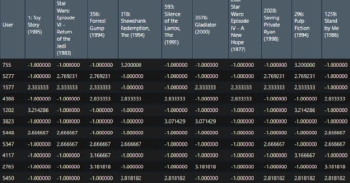
Now it’s time to calculate the recommendation score for each user by iterating over each user and item. In each iteration, first, we’ll calculate the average rating of the user, this will be used in calculating the score, second, we check if the item was rated by user or not, if rated then we store -1 as we are only interested in recommending items that user have not rated or liked.

If the item is not rated then we grab the top 10 items similar to our given item using the similarity matrix we calculated above. Then we fetch the user’s rating for those similar items. We will also calculate the average rating of similar items in order to subtract it with items’ rating.

Finally, we will pass a similar item list, user rating history list for similar items, and an average rating of similar items to our ‘calScore’ score function. The result will be added to the average rating of the user. Doing so will result in scores that will indicate which item to recommend to which users. Higher the score more likely the user will buy that item.

#function to compute score for item recommendation.

calScore <- function(history, similarities,avgRating)

{

return (sum((history-avgRating)*similarities)/sum(similarities))

}

#create empty dataframe for score

data.ibs.user.score = data[FALSE,]

# Loop through the users (rows)

for(i in 1:nrow(data.ibs))

{

#get ratings of the user for each item

ratings <-as.numeric(data.ibs[i,])

#calculate average mean

meanAvg <- mean(ratings[ratings!=0])

#get user id for which to calculate score

users <- as.numeric(data[i,1])

data.ibs.user.score[i,1] <- users

# Loops through the movies (columns)

for(j in 2:ncol(data))

{

# Get the movie's name

item <- colnames(data)[j]

# We do not want to recommend products you have already consumed

# If you have already consumed it, we store -1

#check if user have rated the movie or not.

if(as.integer(data[,c('User',item)] %>% filter(User==users))[-1] > 0)

{

data.ibs.user.score[i,j]<- -1

} else {

# We first have to get a product's top 10 neighbours sorted by similarity

#get top 10 similar movies to our given movie

topN <- head(n=11,( data.ibs.similarity[ order( data.ibs.similarity[,item], decreasing = T),][,c('items',item)] ) )

topN.names <- as.character(topN$User)

topN.similarities <- as.numeric(topN[,item])

#Dropping first movie as it will be the same movie

topN.similarities <- topN.similarities[-1]

topN.names <- topN.names[-1]

# We then get the user's rating history for those 10 movies.

topN.userPurchases <- as.numeric( data[,c('User',topN.names)] %>% filter(User==users))[-1]

#calculate score for the given movie and the user

item.rating.avg<-as.numeric(colMeans(x=data.ibs[,topN.names], na.rm = TRUE))

data.ibs.user.score[i,j] <- meanAvg+(calScore(similarities=topN.similarities,history=topN.userPurchases,avgRating = item.rating.avg))

} # close else statement

} # end product for loop

} # end user for loop

#view scores of each item for users

View(data.ibs.user.score)

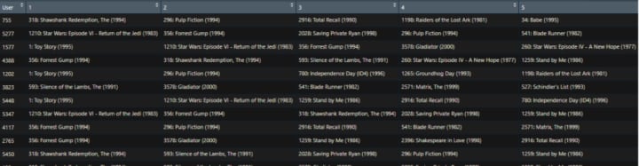
Predicting recommendation scores helps to understand and suggest items but we can further improve how results are shown by replacing scores with the item’s name. Here is how to do it.

#create empty table to store recommended items.

data.user.scores.holder <- read.table(text = "",

colClasses = rep(c('character'),101),

col.names = c('User',seq(1,100)),

check.names = FALSE)

#iterate each rows

for(i in 1:nrow(data.ibs.user.score))

{

#get user id

data.user.scores.holder[i,1]<-data.ibs.user.score[i,1]

#get the names for recommended movies

data.user.scores.holder[i,2:101] <- names(head(n=100,(data.ibs.user.score[,order(as.numeric(data.ibs.user.score[i,]),decreasing=TRUE)])[i,-1]))[1:100]

}

#view recommended items.

View(data.user.scores.holder)

Implementing above will enhance our understanding of how the recommendation system works. But the above code is not efficient and is rather slow. There are many R packages using which we can implement recommendation filtering without any hassle. One such package is recommenderlab.

IBCF Implementation Using Recommender Lab

Now let’s implement IBCF using recommenderLab.

install.packages("recommenderlab")

library(recommenderlab)

recommenderLab works on a ‘real rating matrix’ data set so we have to convert our data frame to it first.

#convert data frame (without user ids) to matrix

data.ibs.matrix <- as.matrix(data.ibs)

#stor user ids as row names of the rating matrix

rownames(data.ibs.matrix) <- data$User

#convert matrix to realRatingMatrix

ratingMatrix <- as(data.ibs.matrix,"realRatingMatrix")

Next, we split our data set into training and test sets. We will be using a training set to build a model for IBCF and evaluate its result on the test set.

#split dataset in to train and test

e <- evaluationScheme(ratingMatrix, method="split", train=0.8, given=5, goodRating=3)

It is time to implement the item-item recommendation system using recommenderLab

#build model with desired parameters

IBCF_Z_P <- Recommender(getData(e, "train"), "IBCF",

param=list(normalize = NULL ,method="cosine"))

And that is it. This one line computed everything that we had implemented above using our own R code.

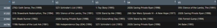
Here is what our model predicted when we provide it train data

#predict items for unknown data

p <- predict(IBCF_Z_P, getData(e, "unknown"), type="topNList", n=5)

as(p,"list") %>% as.data.frame() %>% t()%>% View

Conclusion

Item-item collaborative filtering is a type of recommendation system that is based on the similarity between items calculated using the rating users have given to items. It helps solve issues that user-based collaborative filters suffer from such as when the system has many items with fewer items rated. IBCF is also computationally less intensive than UBCF. Implementing IBCF helps build a strong recommendation system that can be used to recommend items to the users.

Similar Read You May Like

Segment User Based on Their Purchase History